Numerical Methods, High
Performance
Computing
In order to numerically solve complex set of PDEs with solutions
varying on different length scales it is necessary to use advanced
computational methods and perform the calculations on high performance
computers, typically in parallel on many processors.
The single most important factor is to use adaptive mesh refinment
(AMR).
In 3D AMR can speed up the calculations by the factor of millions or
more.
However, even with AMR the calculations can take a very long time on a
single processor (years). Therefore it is also very important to
parallelize
the code so it can exploit the power of multiprocessor supercomputers.
Moreover, the memory requirements for complex simulations can easily
exceed the amount of memory available in any single computational node.
In those cases parallelization is essential (the other alternative is
to use comparatively very expensive shared memory supercomputers).
The Einstein's equations and the relativistic hydro equations are
so complex that the amount of time for communication is negligible
compared to the single step evolution on a patch of domain.
Therefore these calculation can be done on computer clusters
interconnected with high speed networks. The mesage passing interface
(MPI) is designed specifically to work
on distributed memory computers and it is the most widely used
interface for parallel computing today (it also works on shared memory
supercomputers).
My goal is to develop a parallel AMR capable code that will be able to
solve the Einsteins equations coupled with matter modeled by ideal
fluid. This is a collaborative work with Frans Pretorius who has been
very successful with his parallel AMR black hole code in simulating
black hole mergers. The code uses on generalized harmonic coordinates
and free evolution.
There are several groups trying to do just that but I think that it is
essential that there are different independently developed codes on the
"market". Since each code will use a slightly different approach the
probability of generating false results will be greatly
reduced.
I first implemented AMR
for SR hydro in 1D. The idea was to use non-uniform grid (with
hierarchical structure) that would adapt according to some preset
criteria. The time step was global, i.e. it is constrained by the
smallest cell.
1D ideal
fluid simulations
in the test fluid
approximation with AMR
I first tested the AMR algorithm by
evolving a standard shock tube problem and also an initially Gaussian
profile in Minkowski spacetime. Click on the images to see the time
evolution of fluid quantities together with the mesh hierarchy. Note
how
the mesh adjusts to the solution. The criterion used for mesh refinment
was the truncation error estimate.
It can be estimated by performing one step with the mesh coarsened by a
factor of 2 and then compared with two step evolution of the regular
mesh.
 |
 |
Shock tube test -
shown is the
specific internal energy and the mesh hierarchy.
(click to play mpeg movie)
|
Evolution of an
initially smooth
Gaussian pressure profile (with constant initial density and zero
velocity). Pressure, velocity, density and the mesh hierarchy are shown
(from top to bottom).
(click to play mpeg movie)
|
In order to see how the AMR algorithm
handles fluids in strong gravitational fields I tested it by simulating
sperical accretion of an ideal fluid onto a Schwarzschild black hole.
Eddington-Finkelstein ingoing coordinates were used. The inner radius
was set to 0.5M which is well inside the event horizon (2M). The
numerical solution fits the analytic solution perfectly.
I used the AMR code for studying critical
phenomena in fluids.
 |
| Spherical
accretion of perfect
fluid onto a Schwarzschild black hole. Toward the end of the simulation
a stationary state is reached. |
AMR in
2D/3D
Recently I have started working on an
ambitious project that aims to
incorporate hydrodynamics into Frans Pretorius' PAMR/AMRD parallel
infrastructure.
The first task is to develop 2D/3D AMR code based on the Berger and
Oliger algorithm for HRSC methods.
I started with the advection equation since it is the prototype
equation
for conservative systems and is ideally suited for testing and
development.
The algorithm then can be directly aplied for hydrodynamics and that is
currently work in progress.
The Berger and Oliger AMR algorithm is based on hierarchical grid
structure.
The coarsest grid (also known as the base grid) covers the wole
computational domain.
In places where more resolution is needed a finer (child) grid is
created on top of the coarser one (the parent grid).
These grids are layered on top of each other in hierarchical fashion,
i.e., each child
grid is fully contained within a parent grid.
The refinment ratio can be arbitrary but 2 is the most common.
Each grid level uses its own time step satisfying the CFL condition.
This is an important feature of the Berger and Oliger AMR algorithm
that
ameliorates the global time step bottleneck.
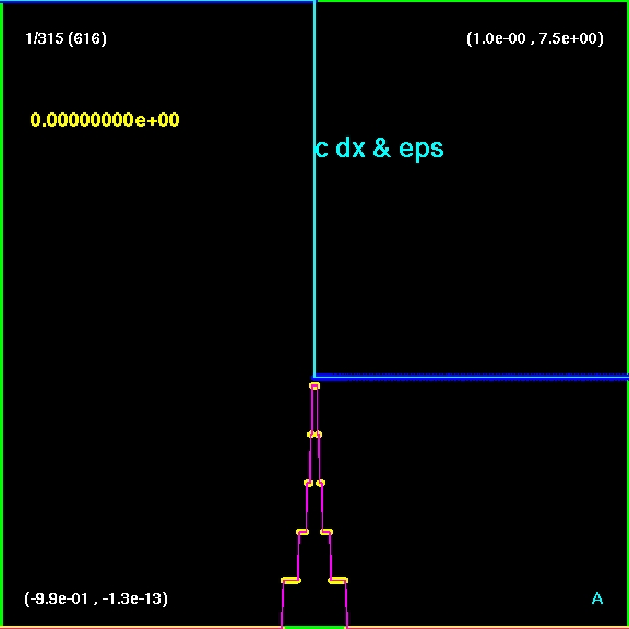
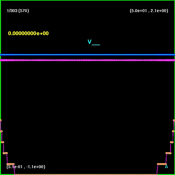
The first image/movie below shows a typical hierarchical 2D grid
structure
taken from an
advection simulation.
Diferent colors represent the different grid hierarchies. By clicking
on the image
a movie will be played that shows the time evolution of the grid
hierarchies.
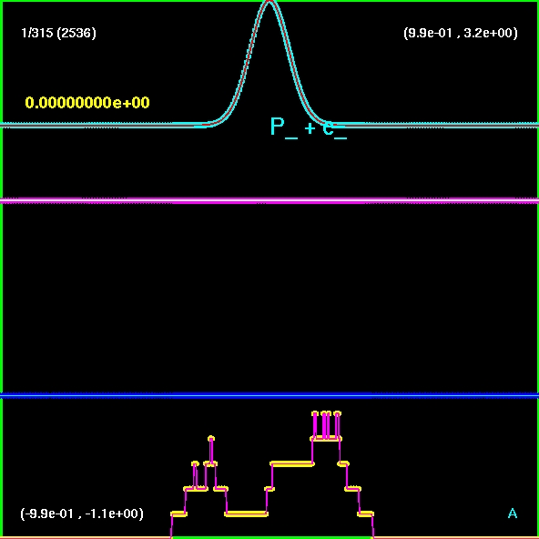
The image/movie on the right shows the actual profile that is being
advected.
The profile consists of two narrow Gaussian peaks. One is rotated so
that there is
no prefered direction in the setup.
The components of the advection velocity are
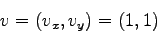 .
.
 |
 |
An example of 2D
hierarchical grid structure. Each child grid is fully contained within
a parent grid. The movie shows the grid evolution during the simulation.
(click to play mpeg movie)
|
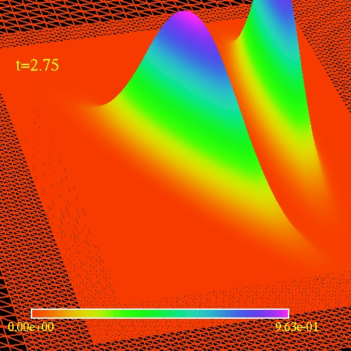
Simulation of an
advection equation using the Berger and Oliger AMR as described in this
section. Four hierarchy levels are visible but there is in fact seven
levels present.
(click to play mpeg movie)
|
The grid hierarchy is
adjusted according to the truncation error
estimate (TRE).
TRE can be estimated by comparing values resulting from substeps on
child grids
with one step on the parent grid.
In order to be able to obtain TRE everywhere one can introduce a
so-called self shadow
hierarchy. It is a child grid that completely covers the base grid.
The Berger and Oliger AMR algorithm was introduced in the context of
finite difference methods.
Although the main principle remains the same also for finite volume
methods there are differences in the detailed implementation.
One important difference is that child grid points overlap with parent
grid
points in finite difference schemes.
In a cell based approach this is no longer true.
Cell averages can be better seen as values at the centers of cells.
Take a cell and divide it into four subcells. It is immediately obvious
that
the center of the parent cell does not coincide with the center of
neither or the
child cells.
This fact must be reflected in interpolation and injection procedures
that
are at the heart of the Berger and Oliger algorithm.
Another difference is that in HRSC methods each step actually consists
of several
Runge-Kutta substeps (for second order methods there are two substeps).
This also must be reflected in the scheme.
Except the technical details there are some conceptual differences as
well.
In fluid dynamics shocks are present and the TRE near shock fronts is
always large.
Therefore the scheme always demands refinement near shocks (this itself
might or might not be desirable). However, shock fronts are
hypersurfaces and that poses a problem for rectangular based grids.
Imagine a line (shock front) stretched diagonaly through a squared
domain.
The child grid that contains the whole line will basically coincide
with the parent grid and that is very ineficcient.
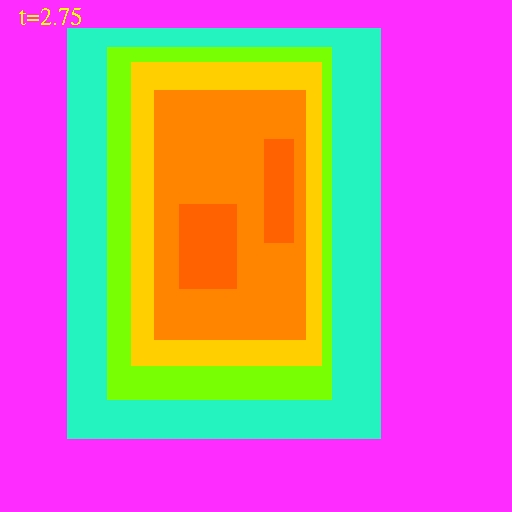
To reduce the inefficiency I introduced the concept of a mask.
Masks are being used in black hole codes to handle singularity
excisions (the singularity inside apparent horizons
can be safely removed from computational domain due to the cosmic
censorship
that is believed to be valid in generic situations).
Here mask marks the cells with high TRE that are to be evolved during
each evolution step.
The rest of the domain will be interpolated from the coarser level.
There are actually two masks - each for each Runke-Kutta substep (I use
second
order scheme therefore two substeps - this can be generalized)
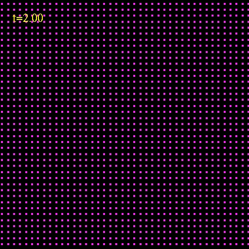
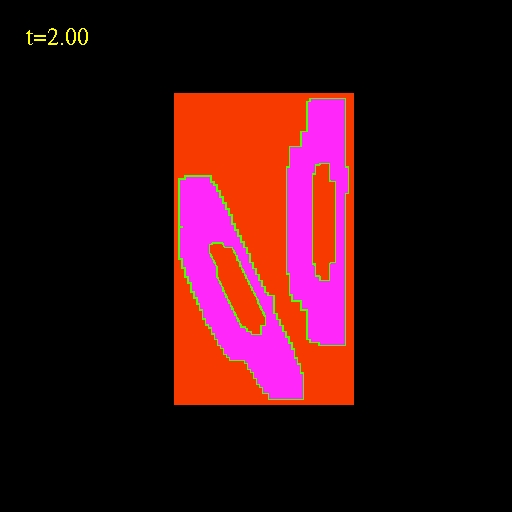
The image bellow shows an example of a mask. The red color (value 0)
represents points
that are not evolved at this level.
Both the green (value 1) and purple (value 3) points are evolved in the
first Runge-Kutta substep but only the purple points are evolved in the
second substep
(the lowest and second lowest bits of the mask identify which points
are to be moved
at each substep).
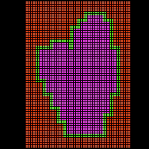 |
| An example of a
mask. The red color (value 0)
represents points
that are not evolved at this level.
Both the green (value 1) and purple (value 3) points are evolved in the
first Runge-Kutta substep but only the purple points are evolved in the
second substep. |
The mask as described above improves the efficiency but one problem
still remains.
Even with the mask present all of the points at the base level will be
evolved.
However, in places where the dynamics is violent and large refinments
are needed the
evolution step will very likely fail.
This is a specific feature of hydrodynamics that is typically not
present in finite
difference codes.
The problem is that the updated conservative variables can easily
assume values
that can not be translated into primitive variables.
However, since at the critical regions the values will be replaced from
injections
from higher levels the cells do not need to be evolved to begin with.
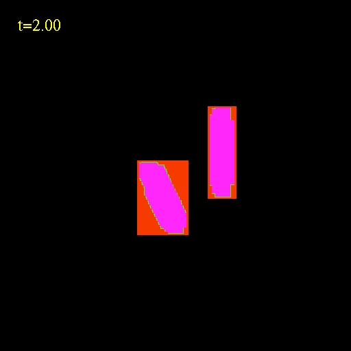
We can therefore cut a "hole" in the mask in place where we expect
injection
from higher levels (some buffering must be retained for the
interpolations to work
properly).
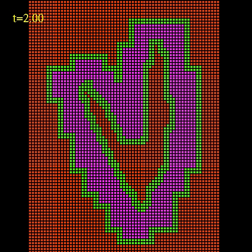
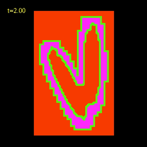
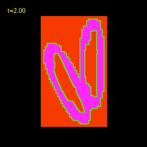
The sequence of images below show the mask at consecutive hierarchies.
This mask sequence is taken directly from the advection simulation
shown in the movie above.
| Sequence of masks
with "holes" in them. The red color (value 0)
represents points
that are not evolved at this level.
Both the green (value 1) and purple (value 3) points are evolved in the
first Runge-Kutta substep but only the purple points are evolved in the
second substep. |