Periodic Boundary Conditions

As a first example, let's consider the linear wave equation in 1 dimension with periodic boundary conditions. The reader familiar with The RNPL Reference Manual will know that RNPL doesn't currently handle periodic boundary conditions. So, we'll get RNPL to produce code and then we'll edit the update routine to provide the correct boundary conditions.

The problem is simple to define. We'll use a left-moving Gaussian pulse for initial data.

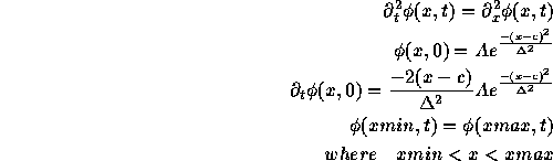
Except for the boundary conditions, this problem is easy to set up using RNPL . We'll use the usual 2nd order leap-frog differencing. The result is:

# This program solves 1D 2nd order wave equation

parameter float xmin := 0
parameter float xmax := 100
parameter float A := 1.0
parameter float c
parameter float delta

rec coordinates t,x

uniform rec grid g1 [1:Nx] {xmin:xmax}

float phi on g1 at -1,0,1

operator D_LF(f,x,x) := (<0>f[1] - 2*<0>f[0] + <0>f[-1])/(dx*dx)
operator D_LF(f,t,t) := (<1>f[0] - 2*<0>f[0] + <-1>f[0])/(dt*dt)

evaluate residual phi { [1:1] := D_LF(phi,t,t) = D_LF(phi,x,x) ;
                     [2:Nx-1] := D_LF(phi,t,t) = D_LF(phi,x,x) ;
                      [Nx:Nx] := D_LF(phi,t,t) = D_LF(phi,x,x) }

initialize phi { [1:Nx] := A*exp(-(x-c)^2/delta^2) }

looper iterative

auto update phi

The residual for can't be left the way it is because the second x derivative would require points at 0 and Nx+1. We save this to a file called wper_rnpl. We can then run the compiler with rnpl -f77 wper_rnpl.

One of the files produced is called updates.f. This file contains:

!----------------------------------------------------------------------
!  This routine updates the following grid functions
!  phi 
!----------------------------------------------------------------------
      subroutine update0(phi_np1,phi_n,phi_nm1,g1_shp,g1_bds,dx,dt)
        implicit none

        include 'globals.inc'

        integer g1_shp(1)
        integer g1_bds(2)
        real*8  phi_np1(g1_bds(1):g1_bds(2))
        real*8  phi_n(g1_bds(1):g1_bds(2))
        real*8  phi_nm1(g1_bds(1):g1_bds(2))
        real*8  dx
        real*8  dt
        integer i,j,k
        integer Nx

        Nx = Nx0 * 2**level + 1

          i=1
            phi_np1(i)=phi_np1(i)-((phi_np1(i)-2*phi_n(i)+phi_nm1(i))/(
     &        dt*dt)-(phi_n(i+1)-2*phi_n(i)+phi_n(i-1))/(dx*dx))/(dt*dt/
     &        (dt*dt*dt*dt))
          do i=2, Nx-1
            phi_np1(i)=phi_np1(i)-((phi_np1(i)-2*phi_n(i)+phi_nm1(i))/(
     &        dt*dt)-(phi_n(i+1)-2*phi_n(i)+phi_n(i-1))/(dx*dx))/(dt*dt/
     &        (dt*dt*dt*dt))
          end do
          i=Nx
            phi_np1(i)=phi_np1(i)-((phi_np1(i)-2*phi_n(i)+phi_nm1(i))/(
     &        dt*dt)-(phi_n(i+1)-2*phi_n(i)+phi_n(i-1))/(dx*dx))/(dt*dt/
     &        (dt*dt*dt*dt))
        return
      end

This routine is easy to modify. We just change the reference to phi_n(i-1) in the first statement to phi_n(Nx). We then change the reference to phi_n(i+1) in the last statement to phi_n(1). The resulting code is:

!----------------------------------------------------------------------
!  This routine updates the following grid functions
!  phi 
!----------------------------------------------------------------------
      subroutine update0(phi_np1,phi_n,phi_nm1,g1_shp,g1_bds,dx,dt)
        implicit none

        include 'globals.inc'

        integer g1_shp(1)
        integer g1_bds(2)
        real*8  phi_np1(g1_bds(1):g1_bds(2))
        real*8  phi_n(g1_bds(1):g1_bds(2))
        real*8  phi_nm1(g1_bds(1):g1_bds(2))
        real*8  dx
        real*8  dt
        integer i,j,k
        integer Nx

        Nx = Nx0 * 2**level + 1

          i=1
            phi_np1(i)=phi_np1(i)-((phi_np1(i)-2*phi_n(i)+phi_nm1(i))/(
     &        dt*dt)-(phi_n(i+1)-2*phi_n(i)+phi_n(Nx))/(dx*dx))/(dt*dt/
     &        (dt*dt*dt*dt))
          do i=2, Nx-1
            phi_np1(i)=phi_np1(i)-((phi_np1(i)-2*phi_n(i)+phi_nm1(i))/(
     &        dt*dt)-(phi_n(i+1)-2*phi_n(i)+phi_n(i-1))/(dx*dx))/(dt*dt/
     &        (dt*dt*dt*dt))
          end do
          i=Nx
            phi_np1(i)=phi_np1(i)-((phi_np1(i)-2*phi_n(i)+phi_nm1(i))/(
     &        dt*dt)-(phi_n(1)-2*phi_n(i)+phi_n(i-1))/(dx*dx))/(dt*dt/
     &        (dt*dt*dt*dt))
        return
      end

We then save the new file and make as usual. Here is an example parameter file:

parameters for wper
lambda := .8
Nx0 := 100
xmin := 0
xmax := 15
level := 0
ser := 0
fout := 1
iter := 1000
epsiter := 1.0e-4
rmod := 10
A := 1.0
c := 5.0
delta := 0.8
in_file := "wp_i0.hdf"
out_file := "wp_o0.hdf"

Unfortunately, due to the trouble with 2nd order initial data discussed in section 1.1, we end up with both a left-moving and a right-moving piece. But the periodic boundary conditions are still apparent as long as the Gaussian is not centered.