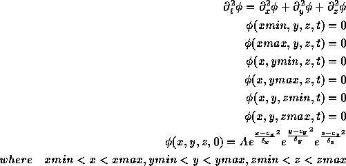


Typically one would also specify  , but we'll ignore this fact for
now. To set this problem up with RNPL we must identify our requirements.
We'll need one grid function
  . We'll need four difference operators
for
  ,
,  ,
,  , and
, and  .
We'll also need parameters for the initial data, namely
  ,
,  ,
,
 , A,
, A,  ,
,  , and
, and  as well as parameters
for the domain boundaries, xmin, xmax, ymin, ymax, zmin, and
zmax.
We begin our RNPL program by specifying the parameters. While RNPL \ statements may appear in any order, it is good for users to keep things organized. Our parameter declarations look like this:
parameter float xmin := 0
parameter float xmax := 100
parameter float ymin := 0
parameter float ymax := 100
parameter float zmin := 0
parameter float zmax := 100
parameter float A    := 1.0
parameter float c_x  := 50.0
parameter float c_y  := 50
parameter float c_z  := 50
parameter float delta_x
parameter float delta_y
parameter float delta_z
Each parameter can be given a default value. There are other parameters the RNPL program will need, but they are automatically defined, so we'll discuss them later.
Next, we define the coordinate system. The declaration looks like this:
rect coordinates t,x,y,z
The name rect is the name of the coordinate system. We can now define a grid which uses these coordinates.
uniform rect grid g1 [1:Nx][1:Ny][1:Nz] {xmin:xmax}{ymin:ymax}{zmin:zmax}
We will define our grid function to have three time levels so we can use the standard leap-frog operators to solve the equation. The definition is:
float phi on g1 at -1,0,1
Now comes the operator definitions. We need four second derivatives, one for each coordinate.
operator D_LF(f,t,t) := (<1>f[0][0][0] - 2*<0>f[0][0][0] +
<-1>f[0][0][0])/(dt*dt)
operator D_LF(f,x,x) := (<0>f[1][0][0] - 2*<0>f[0][0][0] +
<0>f[-1][0][0])/(dx*dx)
operator D_LF(f,y,y) := (<0>f[0][1][0] - 2*<0>f[0][0][0] +
<0>f[0][-1][0])/(dy*dy)
operator D_LF(f,z,z) := (<0>f[0][0][1] - 2*<0>f[0][0][0] +
<0>f[0][0][-1])/(dz*dz)
Since we wish RNPL to produce the complete program, we must specify the partial-differential equations. This is done by defining the residual.
evaluate residual phi {
            [1:Nx][1:Ny][1:1] := <1>phi[0][0][0] = 0;
          [1:Nx][1:Ny][Nz:Nz] := <1>phi[0][0][0] = 0;
            [1:Nx][1:1][1:Nz] := <1>phi[0][0][0] = 0;
          [1:Nx][Ny:Ny][1:Nz] := <1>phi[0][0][0] = 0;
            [1:1][1:Ny][1:Nz] := <1>phi[0][0][0] = 0;
          [Nx:Nx][1:Ny][1:Nz] := <1>phi[0][0][0] = 0;
     [2:Nx-1][2:Ny-1][2:Nz-1] := D_LF(phi,t,t) = D_LF(phi,x,x) +
                                 D_LF(phi,y,y) + D_LF(phi,z,z)
                       }
The boundary conditions could also have been stated with a time derivative of phi, but this would have required another operator definition. The above method is the simplest.
To get RNPL to generate the initial data, we must provide an initialization for phi.
initialize phi {
  [1:Nx][1:Ny][1:Nz] := A*exp(-(x-c_x)^2/delta_x^2)*
                          exp(-(y-c_y)^2/delta_y^2)*
                          exp(-(z-c_z)^2/delta_z^2)
               }
We now instruct RNPL to solve the equation iteratively and to automatically generate the update routine.
looper iterative

auto update phi
Save the program to a file named wave3d_rnpl. The RNPL compiler can now produce C or FORTRAN code with one of the following commands.
rnpl -c wave3d_rnpl
rnpl -f77 wave3d_rnpl
We can produce a makefile for this program using a utility included with the RNPL distribution.
Before we can run the program, we need to create a parameter file. Here is an example:
parameters for wave3d
tag := "3d_"
lambda := .3
Nx0 := 32
Ny0 := 32
Nz0 := 32
xmin := 0
xmax := 10
ymin := 0
ymax := 10
zmin := 0
zmax := 10
ser := 0
fout := 1
iter := 10
epsiter := 1.0e-5
rmod := 1
A := 1.0
c_x := 5.0
c_y := 5
c_z := 5
delta_x := .8
delta_y := .8
delta_z := .8
in_file := "w3d_in.hdf"
out_file := "w3d_out.hdf"
level:=0
Along with the parameters we defined are some automatically defined parameters. See the Reference Manual for more information. Save this to a file called w3d_0.
The program can now be executed with the following command:
wave3d w3d_0
As stated earlier, the initial data should be specified with values for
both  and
and  . Since we've only specified
  , we have
little control over the initial data. RNPL generates a second time level
of data using an iterative procedure over which the user has no control.
So how could we get proper initial data? One was is to write a separate
program for generating initial data from user defined parameters. The only
(current) way for RNPL to generate ``good'' initial data is to reduce the
problem to 1st order form and specify data for the two derivatives of
 . This approach is taken in the next section.


