


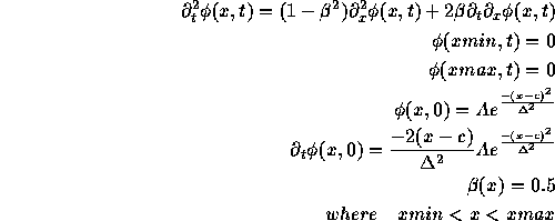
As a slightly more complicated example, let's consider the ``shifted'' wave
equation in 1 dimension. We'll take the shift  to be a constant and
the initial field configuration
to be a constant and
the initial field configuration  to be a left-moving Gaussian pulse.
We'll fix the field values to 0 at the end points. This problem can be
stated as follows:
to be a left-moving Gaussian pulse.
We'll fix the field values to 0 at the end points. This problem can be
stated as follows:
We can rewrite this equation in first order form by introducing the two
auxilliary variables  and
and  defined by:

In terms of these variables, the problem becomes:
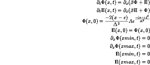
The boundary conditions are a bit tricky, but these seem to work. Below is an RNPL program to solve this problem. This program must be modified if FORTRAN output is desired since FORTRAN is not case sensitive. We use a 2 level Crank-Nicholson difference scheme.
# This program solves 1D 1st order shifted wave equation

parameter float xmin := 0
parameter float xmax
parameter float epsdis
parameter float c
parameter float A
parameter float delta

rec coordinates t,x
uniform rec grid g1 [0:Nx-1] {xmin:xmax}

float Phi on g1 at 0,1
float Pi on g1 at 0,1
float beta on g1 at 0,1
float phi on g1 at 0,1

operator D_FW1(f,x) := (<1>f[1] - <1>f[0])/dx
operator D_FW12(f,x) := (-3*<1>f[0] + 4*<1>f[1] - <1>f[2])/(2*dx)
operator D_BW12(f,x) := (3*<1>f[0] - 4*<1>f[-1] + <1>f[-2])/(2*dx)
operator D_CN(f,t) := (<1>f[0] - <0>f[0])/dt
operator D_CN(f,x) := (<1>f[1] - <1>f[-1] + <0>f[1] - <0>f[-1])/(4*dx)
operator D_CND(f,t) := (<1>f[0] - <0>f[0] +
             epsdis/16*(6*<0>f[0] + <0>f[-2] + <0>f[2] -4*(<0>f[-1] +
<0>f[1])))/dt
operator AVG(f,t) := (<1>f[0] + <0>f[0])/2
operator AVG(f,x) := (<0>f[0] + <0>f[-1])/2

evaluate residual Phi { [0:0] := D_FW12(Phi,x) = 0 ;
                        [1:1] := D_CN(Phi,t) = D_CN(beta*Phi + Pi,x);
                     [2:Nx-3] := D_CND(Phi,t) = D_CN(beta*Phi + Pi,x);
                  [Nx-2:Nx-2] := D_CN(Phi,t) = D_CN(beta*Phi + Pi,x);
                  [Nx-1:Nx-1] := D_BW12(Phi,x) = 0 }

residual Pi { [0:0] := <1>Pi[0] = 0 ;
              [1:1] := D_CN(Pi,t) = D_CN(beta*Pi + Phi,x);
           [2:Nx-3] := D_CND(Pi,t) = D_CN(beta*Pi + Phi,x);
        [Nx-2:Nx-2] := D_CN(Pi,t) = D_CN(beta*Pi + Phi,x);
        [Nx-1:Nx-1] := <1>Pi[0] = 0 }

residual beta { [0:Nx-1] := <1>beta[0] = <0>beta[0] }

residual phi { [0:0] := phi = 0 ;
            [1:Nx-1] := D_FW1(phi,x) = AVG(<1>Phi[0],x) }

initialize beta { [0:Nx-1]:= .5 }
initialize Phi { [0:Nx-1]:= -2*(x-c)/delta^2*A*exp(-(x-c)^2/delta^2) }
initialize Pi { [0:Nx-1]:= -2*(x-c)/delta^2*A*exp(-(x-c)^2/delta^2) }
initialize phi { [0:Nx-1]:= A*exp(-(x-c)^2/delta^2) }

looper iterative

auto update Phi, Pi
auto update beta, phi
A parameter file for the resulting programs is:
lambda := .5
Nx0 := 200
level := 0
xmin := 0
xmax := 50
ser := 0
fout := 1
iter := 400
epsiter := 1.0e-5
epsdis := .8
rmod := 10
A := 1.0
c := 25.0
delta := 4.0
in_file := "w_in0.hdf"
out_file := "w_out0.hdf"
Although rather simple, this program illustrates the use of multiple grid functions and implicit updates.