# Filename: polyinterp.mws

# Creator: Kesten Broughton

# ID: 59073916

# Date: Sept. 25, 2000

#

# Polynomial approximation of functions is an important tool in mathematical physics.

# This worksheet shows the development of the source code for the Lagrange interpolating polynomial.

#

> l1 := [[0,1],[2,3],[4,5]];

# The 'seq' operator constructs sequences

> seq(i^2, i=1..4);

# To extract a subsequence

> seq(op([i,2],l1), i=1..3);

# The 'op' operator is quite complex - see the maple help file - but basically, it can extract a part of an expression.

# In this case we will use it to extract the first value (x-coordinate) of the second element in the list above.

> op([2,1], l1);

# To get Maple to display the functions in this worksheet nicely, it is necessary to initialize ldata. (See below on 'nops').

> ldata := l1;

>

# We use the 'nops' operator to find the number of elements in the 'top level' of an argument. Again, nops is a powerful

# but complex function -> see the help files for much much more.

> nops(l1);

> polyinterp := proc(ldata::list(list)), var::name)

# Declare n = number of data points

> n := nops(ldata);

# This is the main reason why we can't get really nice# echo'ed output from Maple all the way through the worksheet.

# According to maple, nops ( ldata) = 1, I guess since at the moment it is simply a variable with no substructure.

# Unfortunately, this means that all our sequences i=1..n below
# evaluate immediately to i=1 which isn't too interesting when you're trying to imagine the product of 50 terms.
# I would love to find a way to make maple consider that ldata may be filled with many littler things at a later time. ???????
# For now, I will proceed taking this short three term data list above as an example.

> # extract the sequence of x values from ldata

> sx := seq(op([i,1], ldata), i=1..n);

# extract the sequence of function values from ldata

> sf := seq(op([i,2], ldata), i=1..n);

# This akward looking expression is simply all the product of all (x - x[k]) except for (x-x[i]).

> num[i] := product((var-sx[j]), j=1..i-1)*product((var-sx[j]),j=i+1..n);

# This equally ugly looking puppy is the product of (x[i]-x[k]) except for k = i.

> den[i] := product((sx[i]-sx[j]), j=1..i-1)*product((sx[i]-sx[j]), j=i+1..n);

# Now we form the Lagrange coefficients, degree n-1 polynomials which magically evaluate to L[i] = 1 if x = x[i]

# and L[i] = 0 if x = x[k]. Who knows what it's doing at the other points between xmin and xmax but at least it

# behaves very sweetly on our data points.

> L[i] := num[i]/den[i];

> subs(var=x,i=2,L[i]);

> expand(%);

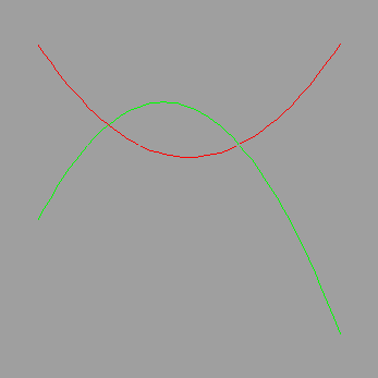
# Let's see what these strange Lagrange polynomial beasts look like. By construction,

# L[2] should equal 1 when x = 2 and 0 at x = 1, 3. Similarly for the others.

# Imagine where the third one goes ...

> plot([subs(var=x, i=1, L[i]), subs(var=x, i=2, L[i])], x=0..6);

# Now remember, these Lagrangian polynomials aren't the final answer. The interpolating polynomial is a linear

# sum of these Lagrangians with coefficients = the f(x[i]).

> p := sum(L[i]*sf[i], i=1..n);

> plot(subs(var=x,p), x=0..6);

# A straight line !!?? I didn't expect that! But if you look back at the data for ldata = l1 you see that it is indeed linear.

# Good work Lagrange!

>