Physics 329: Introduction to Computational Physics:
Software Availability and Usage Hints
This document will be updated throughout the course
Index
General purpose system and programming software
Postscript viewer and plotting software
Visualization and related software
Scientific word-processing and related software
General purpose graphics software and examples
X Windows: As the man page says, X is a
"portable, network-transparent window system". It is the main
windowing system used in most Unix environments. You will
automatically use X when you login to one of
the Phys. Dept. linux machines, or one of the Center for
Relativity SGI machines. To use X on the PCs in the
PMCL follow these instructions:
- login
- double click on the Internet Applications icon
- in the Internet Applications panel, double click on the
XServer icon
- an Xapplication Starter window should pop up. IGNORE
OR CLOSE THIS WINDOW.
- Put the cursor on eXodus in the tool bar on the bottom
of the screen. Click the right mouse button to bring up a menu
and select Login using XDM
- In the XDM Login window which appears, type in the name of the
host to which you wish to connect using X
(
einstein, linux1, etc.), then type or click
CONNECT
- The remote host's login window should appear; login as usual.
(You will have to put the cursor in the login window and click
with a mouse button before you can start typing in the window.)
If the login is successful, in a few seconds
you should see the usual components of an X-session on the remote
machine.
(These components will be superimposed on the usual Windows screen.)
For example, on
einstein you should see a "toolchest"
labelled Desk 1 in the upper left of the screen, as well as
an xterm window.
At this point you can
start additional X-applications (xmaple, more
xterms etc.) from the xterm window, or from the
toolchest.
- Once you have established a session on the remote host via X, you can also
connect to other hosts (using the telnet icon
in Network Applications for example), set the
DISPLAY
environment variable appropriately, e.g.
einstein % setenv DISPLAY pmcl-pc8.ph.utexas.edu:0.0
and start X-applications from there. Note that the Internet address
of each machine should be taped to the system's monitor.
- Don't forget to log out of the remote X-session when you are
through. For example, if logged into
einstein,
choose Log out from the Desktop menu of the toolchest.
A notifier asking you to confirm the log out should appear---click
Yes to log out. A less graceful way to exit is to choose
Close from the eXodus menu.
Maple:
One of the two major general-purpose "symbolic manipulation"
packages (also general-purpose programming environments),
and the one that we will study in this course (the other package
is Mathematica).
On the SGIs type
% xmaple
for the GUI version (in which case make sure your DISPLAY environment
variable is set correctly if running on a remote machine), or
% maple
for a terminal-based (text) session. In the latter instance you
should see something like this.
% maple
    |\^/|     Maple V Release 5 (University of Texas at Austin)
._|\|   |/|_. Copyright (c) 1981-1997 by Waterloo Maple Inc. All rights
 \  MAPLE  /  reserved. Maple and Maple V are registered trademarks of
 <____ ____>  Waterloo Maple Inc.
      |       Type ? for help.
>
If there is any sequence of Maple commands that
you find yourself typing at the beginning of each session (maple
or xmaple) you can put them in a file .mapleinit
in your home directory, whereafter they will automatically be executed
each time you use Maple.
Fortran 77: A general purpose programming language which
is particularly well-suited to numerical (scientific/engineering)
applications. On Unix systems, such as SGI IRIX, the Fortran 77
compiler is often called f77.
Typical usage (on the SGIs):
% f77 -n32 -g mypgm.f mysubs.f -o mypgm
See the
on-line notes
describing the use of Fortran and C in the Unix
environment for additional information.
C: Another general purpose programming language which
is also widely-used for scientific and engineering applications.
On Unix systems the C
compiler is often called cc.
Typical usage (on the SGIs):
% cc -n32 -g mypgm.c myfcns.c -o mypgm
See the
on-line notes
describing the use of Fortran and C in the Unix
environment for additional information.
libp329fa: Utility library for Fortran 77 programs. Available
on SGIs and Crays.
Sample driver for utility routines:
p329fsa.f.
See
source
code
and course notes for further information.
Typical usage:
% f77 pgm.f -L/usr/localn32/lib -lp329 -o pgm
ghostview: Available on SGIs and Linux machines. Use for
viewing Postscript documents. This is an X-application. As with
any X-application, if you are running ghostview on a
remote machine, be sure to set your DISPLAY environment variable so
that your local display is used.
Typical usage (assuming a remote login to einstein from
one the Physics Linux machines):
   einstein% set DISPLAY linux1.ph.utexas.edu:0
   einstein% ghostview somefile.ps
Note: Not all Postscript files will have .ps extensions,
but many do by convention.
gnuplot: X-application available on SGIs and Linux machines.
Use for generating X-Y (2D) and some surface plots. Has extensive
on-line documentation: type help at the
gnuplot prompt for help.
Typical usage:
   einstein% gnuplot
             .
             .
             .
   Terminal type set to 'x11'
   gnuplot> help
             .
             .
             .
   gnuplot> quit
sm: Supermongo plotting package. Available on SGIs.
An alternative to gnuplot
which is somewhat quirkier but generally produces more
professional-looking (i.e. publication-quality) plots. See
on-line
postscript documentation
and on-line help
(type help at the the sm command prompt) for further details.
Supermongo runs as an X-application provided the device
is set to x11.
Ignore the "Can't find entry for iris-ansi-net ..."
message at start-up.
Typical usage:
   einstein% sm
   Can't find entry for iris-ansi-net in /usr/local/lib/sm/termcap
   Hello Matt, please give me a command
   : device x11
   : help
             .
             .
             .
   : quit
vsxynt: A Fortran- and C-callable routine which was
specifically designed for the output and subsequent visualization of data
generated in the solution of time-dependent problems in one spatial
dimension.
Use of this routine in Fortran is illustrated by
the code
vswave.f
which generates a time-series of waveforms,
and, at each time step, outputs the data using vsxynt.
Note that this program is essentially identical to the
gpwave.f
example discussed in class, we're just changing
the "output interface".
Depending on which library is linked-to, data which is
output via vsxynt will be sent to special-purpose files,
or sometimes directly to a visualization server such as
scivis. I strongly recommend that you use the
following libraries when using the vsxynt interface:
-lsvs -lrnpl -lmfhdf -ldf -ljpeg -lz -lsv -lm
I further recommend that you communicate these libraries to make
using the following setenv command which should be placed
in your .cshrc:
setenv LIBVS '-lsvs -lrnpl -lmfhdf -ldf -ljpeg -lz -lsv -lm'
If you do this, then Makefiles such as
this one will work properly.
Assuming that your executable has linked to the libraries given
above, calls to vsxynt will direct data to files with the
extension .sdf. Thus, in the
vswave.f
example, the call
call vsxynt('wave',t,x,y,nx)
will send data to
wave.sdf
.sdf files can then be sent to
scivis
using the
sdftosv
command, as discussed in more detail below.
Important:
Note that .sdf files are not ``human-readable'', so
please don't try to edit them or, worse, to print them!
scivis (jser):
A package for interactive & collaborative
visualization developed at NPAC in Syracuse. Some documentation
is available from the
Scivis home page
and the
User's Guide, but the following should help get you going.
PLEASE SEND ME
E-MAIL
IMMEDAITELY IF YOU HAGE PROBLEMS WITH THIS SOFTWARE.
Assuming that you have established an X session to
einstein, you should be able to start the scivis
visualization server (also known as jser) by selecting
jser from the Tools sub-menu of the toolchest
in the upper left corner of the screen.
Alternatively, you can start jser from the command-line:
einstein% jser &
Note, that we start jser in the background so that we
can continue to type commands at the shell prompt. Note that
jser is an X-application, so be sure that the DISPLAY
environment variable points to your local screen.
Whichever way you start jser, the following window should
pop up on your screen in a few seconds (but be patient, it may be
15 seconds, or so):
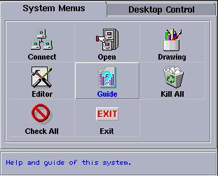
Note that, with the exception of the Exit button---which
shuts the server down---you will probably find little use for the various
selections on the server panel. Rather, you will primarily interact
with the server through additional windows which display
data sets which are sent to the server after it is started. For example,
assume that we have previously generated an .sdf
file using, for example, a Fortran program which calls
vsxynt:
   einstein% pwd
   /usr2/people/phy329/fd/new_wave

   einstein% ls
   Makefile   gpwave.f   vswave.f

   einstein% make vswave
      f77 -g -n32 -c vswave.f
      f77 -g -n32 -L/usr/localn32/lib vswave.o -lp329f \
          -lsvs -lrnpl -lmfhdf -ldf -ljpeg -lz -lsv -lm -o vswave
   ld32: WARNING 84: /usr/localn32/lib/libjpeg.a is not used for ...

   einstein% vswave
    usage: vswave

   einstein% vswave 101

   einstein% ls *.sdf
   wave.sdf
Then, once we have started the scivis server, we can send
the data in this .sdf file to the server using the
sdftosv command:
einstein% sdftosv wave
In a few seconds you should see a window such as the following pop-up:
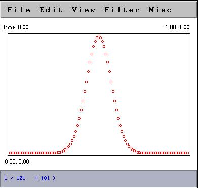
Observe that the new window displays one time step (dataset) of the data
at a time. Using the pull down menus and/or
keyboard accelerators,
you can step through the data, zoom-in or or, play (animate) the data, and
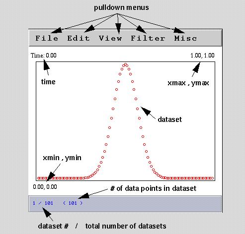
perform many other functions, many of which are fairly self-explanatory.
Here is a guide to the annotations on the above scivis data window:
Note that the server's main function (in the context of this course)
is to provide you with a useful tool to develop and analyze programs
which solve time-dependent partial differential equations in one
spatial dimension (or time
dependent particle motion in 2 dimensions). In particular, you
should not expect to use it to produce ``quality'' hardcopy output.
scivis (jser) keyboard-accelerators
Important Note: Due to a bug in SGI's implementation of Java,
you must first RESIZE any window that scivis creates in
order for the following keyboard accelerators to work. All accelerators
are Ctrl-key based; for example, C-a means depress the ctrl
key and then the a key (without releasing the ctrl key).
| Keystroke |
Mnemonic |
Function |
| C-q
| Quit
| Closes window
|
| C-a
| Animate
| Starts animation
|
| C-s
| Stop
| Stops animation
|
| C-n
| Next
| Displays next dataset
|
| C-p
| Previous
| Displays previous dataset
|
| C-g
| Goto
| Goto specific dataset
|
sdftosv: Sends data in .sdf files to the
Scivis server (also known as jser). Here is the
full usage for the command
   % sdftosv
sdftosv version: 1.0
  Copyright (c) 1997 by Robert L. Marsa
  sends .sdf files to the scivis visualization server
Usage:
  sdftosv [ -i ivec ]
          [ -n oname ]
          [ -s ]
          input_file [ input_file [ ... ] ]

  -i ivec  -- use ivec (0 based) for output control
  -n oname -- name all data sets oname
  -s       -- send data sets one at a time
              useful for large or nonuniform data
  input_file is an .sdf file
Beware that there is a command sdftovs which sends
an .sdf file to a different server---if you get an
error message such as
  assign_Server: Could not communicate with einstein
  assign_Server: Ensure that server is running on einstein and/or
  assign_Server: check/reset value of environment variable VSHOST.
you have typed sdftovs instead of sdftosv.
A typical invocation will be:
   % ls
   wave.sdf

   % sdftosv wave
Note that you do not have to specify the .sdf extension
explicitly, but you can if you so wish.
If we wanted to send only every second time step of wave.sdf
to the server we could use
% sdftosv -i '0-*/2' wave
In this example, the construct
0-*/2
is an example of an index-vector (or ivec), which
is just a shorthand for a regular sequence of integers:
min-max/step ===> min, min + step, min + 2 step, ... min + n step
where n is the largest integer such that
min + n step <= max
Index 0 refers to the first time level of data stored in the
file, and an asterisk (*) can be used in place of min
and/or max to denote "first time-level" or "last time-level"
respectively. When using * in an index-vector specfication,
such as in the above example, be sure to enclose the index-vector in
single quotes to keep the shell from interpreting * in
its own special way.
jv1: Filter which reads two columns of numbers
((x,y) pairs) from standard input and then sends the data to
scivis (jser).
Typical usage:
% jv1 < data_file
or
% jv1 name < data_file
where data_file is a two column file containing the data to
plot. In the first instance, the data will be visualized in a
jser window named Standard input, in the second the
jser window will be labelled name.
libbbhutil.a:
Fortran- and C-callable output utility routines written
for the
Binary Black Holes Grand Challenge Project.
Available on SGIs and HPCF Cray machines. Postscript ``man-style''
documentation for the C routines is available
here.
Fortran routines have the same names (gft_out_bbox etc.)
and can be either called, or invoked as integer functions.
For output of 2- and 3-D arrays on uniform finite-difference meshes, the
routines
gft_out_bbox
should suffice. Here is a usage example:
      integer      nx,        ny
      parameter  ( nx = 65,   ny = 33 )

      real*8       gfcn(nx,ny)
      real*8       xmin,      xmax,     ymin,     ymax,
     &             time

      integer      shape(2),  rank
      real*8       bbox(4)
               .
               .
               .
c------------------------------------------------------
c     'bbox' defines 'bounding box' of coords.
c     associated with the data:
c
c     bbox := ( xmin, xmax, ymin, ymax )
c------------------------------------------------------
      bbox(1) = xmin
      bbox(2) = xmax
      bbox(3) = ymin
      bbox(4) = ymax

      rank = 2
      shape(1) = nx
      shape(2) = ny

      do it = 1 , nt
              .
              .
              .
c------------------------------------------------------
c     The first (string) arg. to 'gft_out_bbox'
c     is stripped of non alphanumeric/underscore
c     characters (including punctuation) if necessary,
c     and then used as the 'stem' for a filename of
c     the form 'stem.sdf'.  All calls to 'gft_out_bbox'
c     with the same string result in output to the
c     same file.
c------------------------------------------------------
         time = it * 1.0d0
         call gft_out_bbox('gfcn',time,shape,rank,
     &                      bbox,gfcn)
      end do
              .
              .
              .
The gft_ routines use
a machine-independent binary format; thus data output using
gft_out_bbox on a Cray, for example, can be processed on
an SGI. On the SGIs, 2- and 3-D data is best visualized using
IRIS Explorer.
A locally developed module, called
ReadSDF_GFT0,
is available for Explorer input of data written using the
gft_ routines.
Here's an
image
of an Explorer map which uses this module.
IRIS Explorer:
A powerful scientific visualization system available on the Center
SGI machines, including einstein. You need to be
logged into einstein via the graphics console to use
the software. Complete documentation for the system
is available via the Online Books selection of the
pull-down Help menu which should appear in the "Toolchest"
located in the upper right corner of the screen when you login.
To use, simply type
% explorer
Here are links to the
IRIS Explorer Center and
Postscript versions of the User's Guide
with graphics
and
without graphics.
latex and tex: Available on SGIs. Scientific
typesetting software. Converts .tex source files
to .dvi files which can then be previewed using
xdvi, or converted to postscript using dvips.
Typical usage:
   % ls
   document.tex

   % latex document.tex
   This is TeX, Version 3.14159 (C version 6.1)
   (document.tex
   LaTeX2e <1996/06/01>
   Hyphenation patterns for english, german, loaded.
             .
             .
             .
   No file document.aux.
   [1] (document.aux) )
   Output written on document.dvi (1 page, 696 bytes).
   Transcript written on document.log.

   % ls
   document.aux   document.dvi   document.log   document.tex
You can easily include Encapsulated Postscript files in a TeX/LaTeX
document, using the epsf package. Here is a sample
tex source file,
here is the
figure file
which is included, and
here is the final
postscript file.
xdvi: X-application for previewing .dvi files (output
from Latex-ing or tex-ing of .tex files). You don't have to
explicitly specify the .dvi extension.
Typical usage:
   % ls
   document.aux   document.dvi   document.log   document.tex

   % xdvi document
dvips: Utility for converting .dvi files to postscript.
Typical usage:
   % ls
   document.aux   document.dvi   document.log   document.tex

   % dvips document
   Got a new papersize
   This is dvips 5.58 Copyright 1986, 1994 Radical Eye Software
   ' TeX output 1997.01.22:1442' -> document.ps
   . [1]

   % ls
   document.aux   document.dvi   document.log   document.ps    document.tex
GLUT: OpenGL Utility Toolkit Programming Interface.
Facilitates construction of OpenGL programs which manipulate
windows, handle user-initiated events etc.
Available PS documentation:
Overview and
Specification/Programmer's Guide.
Typical usage (not all Mesa and X libraries will be required
for all applications):
   % cc -n32 -I/usr/local/include pp2d.c -L/usr/localn32/lib -lglut \
         -lMesaaux -lMesatk -lMesaGLU -lMesaGL -lXmu -lXi -lXext -lX11 \
         -lm -o pp2d
pp2d: OpenGL/X Graphics program for animating two dimensional
particle motion. Currently available
only on Center for Relativity SGI machines, but should display
on any workstation running X (and X-terms).
Typical usage (second form is for monochrome displays):
   % nbody 2.0 0.01 < nbody_input | pp2d
   % nbody 2.0 0.01 < nbody_input | pp2d -m
Help is available via
% pp2d -h
The source code, pp2d.c and
pp2d.h,
may be of interest to those of you interested in using OpenGL
for graphics programming.
Makefile for pp2d.
sphplot: Fortran-callable routine which plots spheres
at a set of specified locations using the SGI GL library.
You must be at an SGI console for this routine to work
Sample Fortran usage
      real*8    positions(3,max_ncharge),   radius
      integer   ncharge

c---------------------------------------------------------
c     Set the radius for *all* displayed spheres.
c---------------------------------------------------------
      radius = 0.03d0

c---------------------------------------------------------
c     Call with ncharge > 0 for normal display.  A graphics
c     window will be opened interactively the first time
c     this routine is called in a program (the outline of
c     a small window will appear on the screen; you will
c     have to position and size the window).
c---------------------------------------------------------
      call sphplot(positions,ncharge,radius)

c---------------------------------------------------------
c     Call with ncharge < 0 (presumably at the end of the
c     simulation) for "tumbling" display.  Depress the escape
c     key in the graphics window to return from the routine.
c---------------------------------------------------------
      call sphplot(positions,-ncharge,radius)
Sample linking and loading with a Fortran main
program pgm.f:
% f77 -g -n32 -c pgm.f
% f77 -g -n32 -L/usr/localn32/lib pgm.o -lp329util -lsphere -lgl -o pgm
Note that sphplot is
part of the p329util library, and that the sphere
and gl libraries must also be linked in.
Here is the source code,
sphplot.c,
and header file,
sphplot.h,
for the routine.