X Windows: As the man page says, X is a "portable, network-transparent window system". It is the main windowing system used in most Unix environments. You will automatically use X when you login to one of the Phys. Dept. X terminals, or the console of one of the Numerical Relativity SGI machines.
Secure Shell (ssh): The basic communication protocol and program which we will use to connect from one machine (such as the Physics Sun Server) to another (such as one of the Numerical Relativity SGIs).
Maple: One of the two major general-purpose "symbolic manipulation" packages (also general-purpose programming environments), and the one that we will study in this course (the other package is Mathematica).
On the SGIs type
sgi1% xmaplefor the GUI version, or
sgi1% maplefor a terminal-based (text) session. In the latter instance you should see something like this.
sgi1% maple
    |\^/|     Maple V Release 5 (University of Texas at Austin)
._|\|   |/|_. Copyright (c) 1981-1997 by Waterloo Maple Inc. All rights
 \  MAPLE  /  reserved. Maple and Maple V are registered trademarks of
 <____ ____>  Waterloo Maple Inc.
      |       Type ? for help.
>
If there is any sequence of Maple commands that
you find yourself typing at the beginning of each session (maple
or xmaple) you can put them in a file .mapleinit
in your home directory, whereafter they will automatically be executed
each time you use Maple.
Fortran 77: A general purpose programming language which is particularly well-suited to numerical (scientific/engineering) applications. On Unix systems, such as SGI IRIX, the Fortran 77 compiler is often called f77.
Typical usage (on the SGIs):
% f77 -64 -g mypgm.f mysubs.f -o mypgmSee the on-line notes describing the use of Fortran and C in the Unix environment for additional information.
C: Another general purpose programming language which
is also widely-used for scientific and engineering applications.
On Unix systems the C
compiler is often called cc.
Typical usage (on the SGIs):
% cc -64 -g mypgm.c myfcns.c -o mypgmSee the on-line notes describing the use of Fortran and C in the Unix environment for additional information.
libp410fa: Utility library for Fortran 77 programs. Available
on SGIs and Linux machines.
Sample driver for utility routines:
p410fsa.f.
See
source
code
and course notes for further information.
Typical usage:
% f77 pgm.f -64 -L/usr/local/lib -lp410 -o pgm
drand48: The Fortran 77 random number function rand, which we discussed in class, and which you used in Homework 3, is SGI-specific.
If you wish to write Fortran code which generates random numbers, but which is portable to (e.g.) Linux systems, I suggest that you use the C routine drand48, which can be called from Fortran through an auxiliary C routine which is defined in this source file:
Note that this source file defines the C-routine drand48_ (i.e. drand48 with an underscore appended). On many Unix systems, including sgi1 and the lnx machines, drand48_ can then be invoked from Fortran via
      real*8      drand48

      write(0,*) 'Here is a random number ', drand48()
Observe that from the point of view of Fortran, the name of the random-number
routine is drand48, NOT drand48_.
Here is the source code, tdrand48.f and Makefile for a sample Fortran 77 program which uses drand48.
If you intend to use this facility, note that you will generally have to do all of the following:
fftpack: A library of Fortran callable routines for performing single and double precision Fast Fourier Transforms (FFTs). Available on sgi1 and lnx machines. Documentation for the double precision routines is available here.
Sample main program tfft.f and Makefile which uses some of the basic routines.
gv: Available on SGIs and Linux machines. Use for
viewing Postscript documents. Largely considered an improved
(more user friendly) version of the venerable ghostview.
Typical usage (assuming a remote login to sgi1 from
one the Physics Xterms):
sgi1% gv somefile.psNote: Not all Postscript files will have .ps extensions, but many do by convention.
ghostview: Available on SGIs and Linux machines. Use for
viewing Postscript documents.
Typical usage (assuming a remote login to sgi1 from
one the Physics Xterms):
sgi1% ghostview somefile.psNote: Not all Postscript files will have .ps extensions, but many do by convention.
gnuplot: X-application available on SGIs and Linux machines.
Use for generating X-Y (2D) and some surface plots. Has extensive
on-line documentation: type help at the
gnuplot prompt for help.
Typical usage:
   sgi1% gnuplot
             .
             .
             .
   Terminal type set to 'x11'
   gnuplot> help
             .
             .
             .
   gnuplot> quit
sm: Supermongo plotting package. Available on SGIs.
An alternative to gnuplot
which is somewhat quirkier but generally produces more
professional-looking (i.e. publication-quality) plots. See
on-line
postscript documentation
and on-line help
(type help at the the sm command prompt) for further details.
Supermongo runs as an X-application provided the device
is set to x11.
Ignore the "Can't find entry for iris-ansi-net ..."
message at start-up.
Typical usage:
   sgi1% sm
   Can't find entry for iris-ansi-net in /usr/local/lib/sm/termcap
   Hello Matt, please give me a command
   : device x11
   : help
             .
             .
             .
   : quit
vsxynt: A Fortran- and C-callable routine which was specifically designed for the output and subsequent visualization of data generated in the solution of time-dependent problems in one spatial dimension.
Use of this routine in Fortran is illustrated by the code vswave.f which generates a time-series of waveforms, and, at each time step, outputs the data using vsxynt. Note that this program is essentially identical to the gpwave.f example discussed in class, we're just changing the "output interface".
Depending on which library is linked-to, data which is output via vsxynt will be sent to special-purpose files, or sometimes directly to a visualization server such as scivis. I strongly recommend that you use the following libraries when using the vsxynt interface:
-lsvs -lrnpl -lsv -lm
I further recommend that you communicate these libraries to make
using the following setenv command which should be placed
in your .cshrc:
setenv LIBVS '-lsvs -lrnpl -lsv -lm'
If you do this, then Makefiles such as
this one will work properly.
Assuming that your executable has linked to the libraries given above, calls to vsxynt will direct data to files with the extension .sdf. Thus, in the vswave.f example, the call
call vsxynt('wave',t,x,y,nx)
will send data to
wave.sdf
.sdf files can then be sent to
scivis
using the
sdftosv
command, as discussed in more detail below.
Important: Note that .sdf files are not ``human-readable'', so please don't try to edit them or, worse, to print them!
scivis (jser): A package for interactive & collaborative visualization developed at NPAC in Syracuse. Unfortunately, the on-line documentation previously available from the NPAC site no longer exists, so if you have any questions concerning the use of the software, contact the instructor.
PLEASE SEND ME E-MAIL IMMEDIATELY IF YOU HAVE PROBLEMS WITH THIS SOFTWARE.
You can start jser from the command-line:
sgi1% jser &Note, that we start jser in the background so that we can continue to type commands at the shell prompt. Also note that jser is an X-application, so even though it is being run on sgi1, the windows should appear on your local screen.
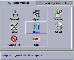
After invocation of jser, the following window should pop up on your screen in a few seconds (but be patient, it may be 15 seconds, or so):
Note that, with the exception of the Exit button---which shuts the server down---you will probably find little use for the various selections on the server panel. Rather, you will primarily interact with the server through additional windows which display data sets which are sent to the server after it is started. For example, assume that we have previously generated an .sdf file using, for example, a Fortran program which calls vsxynt:
   sgi1% pwd
   /usr/people/phys410/fd/new_wave

   sgi1% ls
   Makefile   gpwave.f   vswave.f

   sgi1% make vswave
   f77 -g -64 -c vswave.f
   f77 -g -64 -L/usr/local/lib vswave.o -lp410f -lsvs -lrnpl -lsv -o vswave

   sgi1% vswave
    usage: vswave

   sgi1% vswave 101

   sgi1% ls *.sdf
   wave.sdf
Then, once we have started the scivis server, we can send
the data in this .sdf file to the server using the
sdftosv command:
sgi1% sdftosv waveIn a few seconds you should see a window such as the following pop-up:
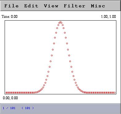
Observe that the new window displays one time step (dataset) of the data at a time. Using the pull down menus and/or keyboard accelerators, you can step through the data, zoom-in or or, play (animate) the data, and perform many other functions, many of which are fairly self-explanatory.
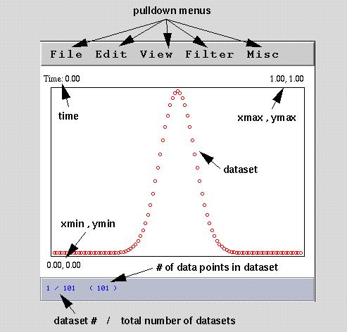
Here is a guide to the annotations on the above scivis data window:
Note that the server's main function (in the context of this course) is to provide you with a useful tool to develop and analyze programs which solve time-dependent partial differential equations in one spatial dimension (or time dependent particle motion in 2 dimensions). In particular, you should not expect to use it to produce ``quality'' hardcopy output.
scivis (jser) keyboard-accelerators
Important Note: Due to a bug in SGI's implementation of Java, you must first RESIZE any window that scivis creates in order for the following keyboard accelerators to work. All accelerators are Ctrl-key based; for example, C-a means depress the ctrl key and then the a key (without releasing the ctrl key).
| Keystroke | Mnemonic | Function |
|---|---|---|
| C-q | Quit | Closes window |
| C-a | Animate | Starts animation |
| C-s | Stop | Stops animation |
| C-n | Next | Displays next dataset |
| C-p | Previous | Displays previous dataset |
| C-g | Goto | Goto specific dataset |
sdftosv: Sends data in .sdf files to the Scivis server (also known as jser). Here is the full usage for the command
   % sdftosv
sdftosv version: 1.0
  Copyright (c) 1997 by Robert L. Marsa
  sends .sdf files to the scivis visualization server
Usage:
  sdftosv [ -i ivec ]
          [ -n oname ]
          [ -s ]
          input_file [ input_file [ ... ] ]

  -i ivec  -- use ivec (0 based) for output control
  -n oname -- name all data sets oname
  -s       -- send data sets one at a time
              useful for large or nonuniform data
  input_file is an .sdf file
Beware that there is a command sdftovs which sends
an .sdf file to a different server---if you get an
error message such as
  assign_Server: Could not communicate with sgi1
  assign_Server: Ensure that server is running on sgi1 and/or
  assign_Server: check/reset value of environment variable VSHOST.
you have typed sdftovs instead of sdftosv.
A typical invocation will be:
   % ls
   wave.sdf

   % sdftosv wave
Note that you do not have to specify the .sdf extension explicitly, but you can if you so wish.
% sdftosv -i '0-*/2' waveIn this example, the construct
0-*/2is an example of an index-vector (or ivec), which is just a shorthand for a regular sequence of integers:
min-max/step ===> min, min + step, min + 2 step, ... min + n stepwhere n is the largest integer such that
min + n step <= maxIndex 0 refers to the first time level of data stored in the file, and an asterisk (*) can be used in place of min and/or max to denote "first time-level" or "last time-level" respectively. When using * in an index-vector specfication, such as in the above example, be sure to enclose the index-vector in single quotes to keep the shell from interpreting * in its own special way.
jv1: Filter which reads two columns of numbers
((x,y) pairs) from standard input and then sends the data to
scivis (jser).
Typical usage:
% jv1 < data_fileor
% jv1 name < data_filewhere data_file is a two column file containing the data to plot. In the first instance, the data will be visualized in a jser window named Standard input, in the second the jser window will be labelled name.
libbbhutil.a: Fortran- and C-callable output utility routines written for the Binary Black Holes Grand Challenge Project. Available on SGIs and HPCF Cray machines. Postscript ``man-style'' documentation for the C routines is available here. Fortran routines have the same names (gft_out_bbox etc.) and can be either called, or invoked as integer functions. For output of 2- and 3-D arrays on uniform finite-difference meshes, the routines
gft_out_bbox
should suffice. Here is a usage example:
      integer      nx,        ny
      parameter  ( nx = 65,   ny = 33 )

      real*8       gfcn(nx,ny)
      real*8       xmin,      xmax,     ymin,     ymax,
     &             time

      integer      shape(2),  rank
      real*8       bbox(4)
               .
               .
               .
c------------------------------------------------------
c     'bbox' defines 'bounding box' of coords.
c     associated with the data:
c
c     bbox := ( xmin, xmax, ymin, ymax )
c------------------------------------------------------
      bbox(1) = xmin
      bbox(2) = xmax
      bbox(3) = ymin
      bbox(4) = ymax

      rank = 2
      shape(1) = nx
      shape(2) = ny

      do it = 1 , nt
              .
              .
              .
c------------------------------------------------------
c     The first (string) arg. to 'gft_out_bbox'
c     is stripped of non alphanumeric/underscore
c     characters (including punctuation) if necessary,
c     and then used as the 'stem' for a filename of
c     the form 'stem.sdf'.  All calls to 'gft_out_bbox'
c     with the same string result in output to the
c     same file.
c------------------------------------------------------
         time = it * 1.0d0
         call gft_out_bbox('gfcn',time,shape,rank,
     &                      bbox,gfcn)
      end do
              .
              .
              .
The gft_ routines use a machine-independent binary format; thus data output using gft_out_bbox on a Cray, for example, can be processed on an SGI. On the SGIs, 2- and 3-D data is best visualized using IRIS Explorer. A locally developed module, called ReadSDF_GFT0, is available for Explorer input of data written using the gft_ routines. Here's an image of an Explorer map which uses this module.
IRIS Explorer: A powerful scientific visualization system available on the Center SGI machines, including sgi1. You need to be logged into sgi1 via the graphics console to use the software. Complete documentation for the system is available via the Online Books selection of the pull-down Help menu which should appear in the "Toolchest" located in the upper right corner of the screen when you login. To use, simply type
% explorer
Here are links to the
IRIS Explorer Center and
Postscript versions of the User's Guide
with graphics
and
without graphics.
latex and tex: Available on SGIs. Scientific
typesetting software. Converts .tex source files
to .dvi files which can then be previewed using
xdvi, or converted to postscript using dvips.
Typical usage:
   % ls
   document.tex

   % latex document.tex
   This is TeX, Version 3.14159 (C version 6.1)
   (document.tex
   LaTeX2e <1996/06/01>
   Hyphenation patterns for english, german, loaded.
             .
             .
             .
   No file document.aux.
   [1] (document.aux) )
   Output written on document.dvi (1 page, 696 bytes).
   Transcript written on document.log.

   % ls
   document.aux   document.dvi   document.log   document.tex
You can easily include Encapsulated Postscript files in a TeX/LaTeX
document, using the epsf package. Here is a sample
tex source file,
here is the
figure file
which is included, and
here is the final
postscript file.
xdvi: X-application for previewing .dvi files (output
from Latex-ing or tex-ing of .tex files). You don't have to
explicitly specify the .dvi extension.
Typical usage:
   % ls
   document.aux   document.dvi   document.log   document.tex

   % xdvi document
dvips: Utility for converting .dvi files to postscript.
Typical usage:
% ls document.aux document.dvi document.log document.tex % dvips document Got a new papersize This is dvips 5.58 Copyright 1986, 1994 Radical Eye Software ' TeX output 1997.01.22:1442' -> document.ps. [1] % ls document.aux document.dvi document.log document.ps document.tex
Open GL: A widely used software interface to graphics hardware, consisting of about 120 commands which are used to specify the objects and operations needed to produce interactive 2- and 3-dimensional applications.
This software is available on sgi1 as well as on lnx[123], but note that since you will generally want to be at a workstation console when programming in OpenGL, you should use lnx[123].
Available PS documentation:
GLUT: OpenGL Utility Toolkit Programming Interface. Facilitates construction of OpenGL programs which manipulate windows, handle user-initiated events etc.Available PS documentation:
See pp2d below for sample application including a Makefile which can be modified for use on sgi1 and lnx[123].Note that the Makefile requires the followinng environment variables to be set as documented HERE.
CC
CCFLAGS
CCCFLAGS
CCLFLAGS
LIBGL
On the lnx machines, these variables should be set properly by default, for all users. On sgi1, you should add them to your
~/.csrhc.
Open Inventor: An object-oriented toolkit (written in C++) that simplifies and abstracts the task of writing graphics programming into a set of easy to use objects.
This software is available on sgi1 as well as on lnx[123], but note that since you will generally want to be at a workstation console when programming in Inventor, you should use lnx[123].
Available documentation: Under construction, in the meantime, start with man inventor.
Part of the Open Inventor environment is ivview, a fast interactive 3D viewer of Inventor files. The source code for this application, ivview.C and ivviewMenus.h may be of interest to those of you interested in using Open Inventor for graphics programming. Makefile for ivview. Sample Inventor File (ASCII format) engine.iv.
Note that the Makefile requires the followinng environment variables to be set as documented HERE.
CXX
CXXFLAGS
CXXCFLAGS
CXXLFLAGS
LIBINVENTOR
On the lnx machines, these variables should be set properly by default, for all users. On sgi1, you should add them to your
~/.csrhc.
pp2d: OpenGL/GLUT Graphics program for animating two dimensional particle motion. Currently available on sgi1 and on lnx[123]. Runs as an X-application on sgi1, but must be used via the console on lnx[123].
Sample usage
   % nbody 2.0 0.01 < nbody_input | pp2d
   % nbody 2.0 0.01 < nbody_input | pp2d -m
Help is available via
% pp2d -hThe source code, pp2d.c, pp2d.h and Makefile, may be of interest to those of you interested in using OpenGL for graphics programming.
Sample 6-body input file input6. Use
% pp2d < input6to view.
XForms: A software package consisting of
This software is available on sgi1 as well as on lnx[123].
Available PS documentation:
See xfpp3d below for sample application including a Makefile which can be modified for use on sgi1 and lnx[123].
pp3d: OpenGL/GLUT Graphics program for animating three dimensional particle motion. Currently available on sgi1 and on lnx[123]. Runs as an X-application on sgi1, but must be used via the console on lnx[123].
Sample usage
   % nbody 2.0 0.01 < nbody_input | pp3d
   % nbody 2.0 0.01 < nbody_input | pp3d -m
Help is available via
% pp3d -hAgain, the source code, pp3d.c, pp3d.h and Makefile may be of interest to those of you interested in using OpenGL for graphics programming.
Sample 20-body input file input20. Use
% pp3d < input20to view.
Warning: This application is still under development. Report
any problems to Matt immediately.
xfpp3d: Version of pp3d which incorporates a GUI created using the XForms package.
Currently available on sgi1 and on lnx[123]. Must be used via the console on all machines.
Sample usage
% nbody 2.0 0.01 < nbody_input | xfpp3d
xfpp3d expects input in precisely the same format as pp3d does.
The source code, xfpp3d_main.c, and Makefile may be of interest to those of you interested in using OpenGL and XForms for graphics programming.
Warning: This application is still under development. Report
any problems to Matt immediately.
E-cell: A package for cellular and biochemical modeling and simulation, which runs under Linux. Available from www.e-cell.org. Currently installed on vnfe1.physics.ubc.ca only. See
/usr/doc/ecell/1.0/on that machine, and the contents therein, for more information. Also see the Rule File Reference Manual (PS)