function fto = barycentric(xfr, ffr, xto)
% fto performs polynomial interpolation using barycentric formula.
%
% Input arguments
%
%  xfr:  x values to fit (length n vector)
%  ffr:  y values to fit (length n vector)
%  xto:  x values at which to evaluate fit (length nto vector)
%
% Output argument
%
%  yto:  Interpolated values (length nto vector)

   % Initialize output ...
   fto = zeros(1, length(xto));

   % Check for consistent length of input arguments ...
   if length(xfr) ~= length(ffr)
      error('Input arguments xfr and ffr must be of same length');
   end

   % Calculate barycentric weights ...
   n = length(xfr);
   w = ones(1,n);
   for j = 1 : n
      for k = 1 : n
         if k ~= j
            w(j) = w(j) * (xfr(j) - xfr(k));
         end
      end
      w(j) = 1.0 / w(j);
   end

   % Perform interpolation to xto values ...
   for k = 1 : length(xto)
      num = 0;
      den = 0;
      for j = 1 : n
         num = num + w(j) * ffr(j) / (xto(k) - xfr(j));
         den = den + w(j) / (xto(k) - xfr(j));
      end
      fto(k) = num / den;
   end
end
clf;
x = linspace(-0.9,0.9,101);
fxct = tpoly(x);
plot(x,fxct);
hold on;
xfr = linspace(-1,1,8);
ffr = tpoly(xfr);
xto = linspace(-0.9,0.9,101);
fto = barycentric(xfr,ffr,xto);
df = fxct - fto
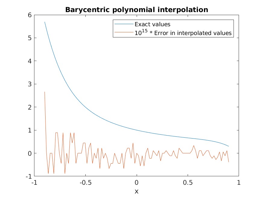
plot(x,1.0e15 .* df);
title('Barycentric polynomial interpolation');
xlabel('x');
legend('Exact values', '10^{15} * Error in interpolated values');
tbarycentric.m
Observe that the error in the interpolated values has been scaled by \( 10^{15} \), which results in values that are \( O(1) \). This indicates that the interpolation error is of the order of machine precision, as we would expect.
pendulum and lpendulumStart a Matlab session and arrange the command window so that you can work in it while viewing these notes, since you'll be doing a lot of cut and pasting in the early part of the lab.
DOWNLOAD SOURCE
pendulum.m (Nonlinear)lpendulum.m (Linear)pendulum solves the nonlinear pendulum equation using
\(O(\Delta t^2)\) finite difference techniques as discussed in class.
As usual, we can examine the function
definition from the Matlab command line using type:
>> type pendulum

function [t theta omega] = pendulum(tmax, level, theta0, omega0)
%  Solves nonlinear pendulum equation using second order finite difference
%  approximation as discussed in class.
%
%  Input arguments
%
%      tmax:   (real scalar) Final solution time.
%      level:  (integer scalar) Discretization level.
%      theta0: (real scalar) Initial angular displacement of pendulum.
%      omega0: (real scalar) Initial angular velocity of pendulum.
%
%  Return values
%
%      t:      (real vector) Vector of length nt = 2^level + 1 containing
%              discrete times (time mesh).
%      theta:  (real vector) Vector of length nt containing computed
%              angular displacement at discrete times t(n).
%      omega:  (real vector) Vector of length nt containing computed
%              angular velocity at discrete times t(n).
%%%%%%%%%%%%%%%%%%%%%%%%%%%%%%%%%%%%%%%%%%%%%%%%%%%%%%%%%%%%%%%%%%%%%%%%%%%

   % trace controls "tracing" output.  Set 0 to disable, non-0 to enable.
   trace = 1;
   % tracefreq controls frequency of tracing output in main time step loop.
   tracefreq = 100;

   if trace
      fprintf('In pendulum: Argument dump follows\n');
      tmax, level, theta0, omega0
   end

   % Define number of time steps and create t, theta and omega arrays of
   % appropriate size for efficiency.
   nt = 2^level + 1;
   t = linspace(0.0, tmax, nt);
   theta = zeros(1,nt);
   omega = zeros(1,nt);

   % Determine discrete time step from t array.
   deltat = t(2) - t(1);

   % Initialize first two values of the pendulum's angular displacement.
   theta(1) = theta0;
   theta(2) = theta0 + deltat * omega0 - 0.5 * deltat^2 * sin(theta0);

   if trace
      fprintf('deltat=%g theta(1)=%g theta(2)=%g\n',...
              deltat, theta(1), theta(2));
   end

   % Initialize first value of the angular velocity.
   omega(1) = omega0;

   % Evolve the oscillator to the final time using the discrete equations
   % of motion.  Also compute an estimate of the angular velocity at
   % each time step.
   for n = 2 : nt-1
      % This generates tracing output every 'tracefreq' steps.
      if rem(n, tracefreq) == 0
         fprintf('pendulum: Step %d of %d\n', n, nt);
      end

      theta(n+1) = 2 * theta(n) - theta(n-1) - deltat^2 * sin(theta(n));

      omega(n) = (theta(n+1) - theta(n-1)) / (2 * deltat);
   end
   % Use linear extrapolation to determine the value of omega at the
   % final time step.
   omega(nt) = 2 * omega(nt-1) - omega(nt-2);
end
lpendulum is a precisely analogous function that solves the
linear pendulum equation (the one you've seen in previous
physics courses) and, apart from comments, diagnostic
messages, and variable name changes, the code for
the two functions differ in literally two lines.
>> type lpendulum

function [t theta omega] = lpendulum(tmax, level, theta0, omega0)
%  Solves linear pendulum equation using second order finite difference
%  approximation.
%
%  Input arguments
%
%      tmax:   (real scalar) Final solution time.
%      level:  (integer scalar) Discretization level.
%      theta0: (real scalar) Initial angular displacement of pendulum.
%      omega0: (real scalar) Initial angular velocity of pendulum.
%
%  Return values
%
%      t:      (real vector) Vector of length nt = 2^level + 1 containing
%              discrete times (time mesh).
%      theta:  (real vector) Vector of length nt containing computed
%              angular displacement at discrete times t(n).
%      omega:  (real vector) Vector of length nt containing computed
%              angular velocity at discrete times t(n).
%%%%%%%%%%%%%%%%%%%%%%%%%%%%%%%%%%%%%%%%%%%%%%%%%%%%%%%%%%%%%%%%%%%%%%%%%%%

   % trace controls "tracing" output.  Set 0 to disable, non-0 to enable.
   trace = 1;
   % tracefreq controls frequency of tracing output in main time step loop.
   tracefreq = 100;

   if trace
      fprintf('In lpendulum: Argument dump follows\n');
      tmax, level, theta0, omega0
   end

   % Define number of time steps and create t, theta and omega arrays of
   % appropriate size for efficiency.
   nt = 2^level + 1;
   t = linspace(0.0, tmax, nt);
   theta = zeros(1, nt);
   omega = zeros(1, nt);

   % Determine discrete time step from t array.
   deltat = t(2) - t(1);

   % Initialize first two values of the pendulum's angular displacement.
   theta(1) = theta0;
   theta(2) = theta0 + deltat * omega0 - 0.5 * deltat^2 * theta0;

   if trace
      fprintf('deltat=%g theta(1)=%g theta(2)=%g\n',...
              deltat, theta(1), theta(2));
   end

   % Initialize first value of the angular velocity.
   omega(1) = omega0;

   % Evolve the oscillator to the final time using the discrete equations
   % of motion.  Also compute an estimate of the angular velocity at
   % each time step.
   for n = 2 : nt-1
      % This generates tracing output every 'tracefreq' steps.
      if rem(n, tracefreq) == 0
         fprintf('lpendulum: Step %d of %d\n', n, nt);
      end

      % Note that the last term is deltat^2 * theta(n), whereas
      % for the nonlinear pendulum it is deltat^2 * sin(theta(n)).
      % This is the ONLY difference in the FDAs for the two
      % systems.

      theta(n+1) = 2 * theta(n) - theta(n-1) - deltat^2 * theta(n);

      omega(n) = (theta(n+1) - theta(n-1)) / (2 * deltat);
   end
   % Use linear extrapolation to determine the value of omega at the
   % final time step.
   omega(nt) = 2 * omega(nt-1) - omega(nt-2);
end
We will first use these functions in tandem so that we can compare the behaviour of the pendulum for the nonlinear/linear cases.
In all of the calculations below, we will start with
theta0 = 0 (i.e. so that the pendulum is hanging vertically),
but will vary the initial angular velocity omega0
Assign values to variables that will be used as input arguments to the functions---be sure to type all of the assignment statements carefully!
Start with a small value of omega0
>> tmax = 40.0
>> level = 8
>> theta0 = 0
>> omega0 = 0.01
Recall that level implicitly defines
via
\[ n_t = 2^{\rm level} + 1 \]
\[ \Delta t = \frac{t_{\rm max}}{2^{\rm level}} \]
so in this case, the solution will be computed at a total of 257 discrete times, including the first and second time steps where the values are determined by the initial conditions.
Now call pendulum, being careful to specify a vector of three names on the left hand side of the assignment so that all output arguments from pendulum are captured
>> [t theta omega]   =  pendulum(tmax, level, theta0, omega0);

In pendulum: Argument dump follows
tmax =  40
level =  8
theta0 = 0
omega0 =  0.010000
deltat=0.15625 theta(1)=0 theta(2)=0.0015625
pendulum: Step 100 of 257
pendulum: Step 200 of 257
Now call lpendulum with the same arguments, but being sure to
use different names on the left hand side for the angular
displacement and velocity , i.e. ltheta and lomega. It
doesn't matter that we use the same name t in the two calls
since the output vector of times is the same for the two calculations.
>> [t ltheta lomega] = lpendulum(tmax, level, theta0, omega0);

In lpendulum: Argument dump follows
tmax =  40
level =  8
theta0 = 0
omega0 =  0.010000
deltat=0.15625 theta(1)=0 theta(2)=0.0015625
lpendulum: Step 100 of 257
lpendulum: Step 200 of 257
Plot the results: note the use of two plot commands with
hold on: recall that the latter tells Matlab not to clear the figure
window each time a plot command is executed
>> clf; hold on; plot(t, theta, 'r'); plot(t, ltheta, 'og');
Observe that the period of the oscillation is \(2\pi\), which follows from our use of "natural units", \(g=L=1\).
Also note how there is very little difference in the motions of the two types of pendula; this is expected since the amplitude is small in this case---about 0.01 radians---so \(\theta\) and \(\sin(\theta)\) are nearly equal at all times
Calculate and plot the actual difference in the \(\theta\)'s between the two simulations.
>> clf; plot(t, theta-ltheta);
Note that the difference is oscillatory, with an amplitude that increases in time---the difference is real, i.e. it is not due to the approximate nature of the solutions but represents the small deviation of the nonlinear pendulum from precisely-linear behaviour.
As a stringent test that our numerical solution is behaving
as it should---implying that the implementation is correct---we
will now perform a basic 3-level convergence test for the nonlinear
pendulum, as discussed in class. That is, we will perform a set of
three calculations where three of the four parameters that we supply
to pendulum, namely
tmaxtheta0omega0are held fixed, while the grid spacing (time step),
\(\Delta t\),
is varied. Again,
keep in mind that we change the time step (by factors of two)
by changing the integer-valued level parameter.
For this test we will use
From this point onward, I recommend that you use "copy and paste" to enter the commands, and to expedite this I will not include the prompt at the beginning of each Matlab command line, This will allow you to select and copy an entire block of commands from your browser, and then paste them into the Matlab session. Just be careful not to copy any of the Matlab output from the command/output block.
However, if you do choose to type the commands manually, be careful with your typing, paying particular attention to the names on the left hand sides of the assignment statements
[t6 theta6 omega6]   =  pendulum(tmax, 6, theta0, omega0);

In pendulum: Argument dump follows
tmax =  40
level =  6
theta0 = 0
omega0 =  0.010000
deltat=0.625 theta(1)=0 theta(2)=0.00625
[t7 theta7 omega7]   =  pendulum(tmax, 7, theta0, omega0);

In pendulum: Argument dump follows
tmax =  40
level =  7
theta0 = 0
omega0 =  0.010000
deltat=0.3125 theta(1)=0 theta(2)=0.003125
pendulum: Step 100 of 129
[t8 theta8 omega8]   =  pendulum(tmax, 8, theta0, omega0);

In pendulum: Argument dump follows
tmax =  40
level =  8
theta0 = 0
omega0 =  0.010000
deltat=0.15625 theta(1)=0 theta(2)=0.0015625
pendulum: Step 100 of 257
pendulum: Step 200 of 257
First, graph \(\theta(t)\) from the 3 calculations on the same plot:
clf; hold on; plot(t6, theta6, 'r-.o');
plot(t7, theta7, 'g-.+'); plot(t8, theta8, 'b-.*');
Note that the curves show general agreement, but that as time progresses there is an increasing amount of deviation, which is most pronounced for the calculation that used the largest grid spacing (level 6, red line)
The observed deviations are a result of the approximate nature of the finite difference scheme
Now, "downsample" the level 7 and 8 theta arrays so that they have the
same length as the level 6 arrays (with values defined at the
times in t6). This means we select every second element of theta7
and every fourth of theta8, which is easy to do using the colon
operator:
theta7 = theta7(1:2:end);
theta8 = theta8(1:4:end);
Now, compute the differences in the grid functions from level to level, assigning them to new variables ...
dtheta67 = theta6 - theta7;
dtheta78 = theta7 - theta8;
and make a plot of the differences.
clf; hold on; plot(t6, dtheta67, 'r-.o'); plot(t6, dtheta78, 'g-.+');
Note that the two curves have the same shape, but different overall amplitudes; each curve is (up to some numeric factor that is approximately 1, i.e. "of order unity") a direct measure of the error in the numerical solution
Now scale (multiply) dtheta78 by 4 and replot together
with dtheta67. If the convergence is second order, the curves should be
nearly coincident (the grid spacing goes down by a factor of 2,
so the differences should go down by a factor of \(2^2 = 4\))
dtheta78 = 4 * dtheta78;
clf; hold on; plot(t6, dtheta67, 'r-.o'); plot(t6, dtheta78, 'g-.+');
Are they nearly coincident?
Also note how the magnitude of the error increases with time, which is characteristic of a finite difference solution of this type
We can extend our convergence test by repeating the calculation
with an even higher level, level = 9.
Again, recall that this means the grid spacing---the discrete time step, \(\Delta t\)---will be reduced by a factor of 2 relative to the level 8 computation.
[t9 theta9 omega9] = pendulum(tmax, 9, theta0, omega0);
Downsample theta9, compute the difference relative to theta8, scale by the appropriate power of 4, which is \(4^2 = 16\), and add to the plot:
theta9 = theta9(1:8:length(theta9));
dtheta89 = theta8 - theta9;
dtheta89 = 16 * dtheta89;
plot(t6, dtheta89, 'b-.*');
Note how the sequence from red -> green -> blue curves shows
increasingly good overlap: this is exactly what we expect, since
as \(\Delta t \to 0\),
i.e. as level \(\to \infty\), the leading
order error term in the finite difference solution
which is \(O(\Delta t^2)\),
will become increasingly dominant over the higher order terms
\(O(\Delta t^4), O(\Delta t^6). \ldots\)
We could continue the convergence test to even higher levels,
level = 10, 11, ... , but we should note that, as
discussed in class, for sufficiently
high level (sufficiently small \(\Delta t\)) the finite difference
approximation would not improve, and, in fact, would begin to
degrade as a result of round off and catastrophic loss of precision.
In any case, from the convergence test, we now have strong evidence that the implementation is correct
We can therefore move on to "doing some science" with the code; ultimately, of course, this is the purpose of any project in computational science
We start by performing simulations using a sequence of increasing
values of omega0 , for fixed tmax and
theta0, and at level = 8.
Physically, this means that we will be giving the pendula ever increasing initial angular velocities, so the resulting amplitude of the motion will also increase.
A key result that you can see immediately is whereas the period (frequency) of the linear pendulum (green) stays constant at \(2\pi\), i.e. is not dependent on the amplitude of the oscillation, the period of the nonlinear pendulum (red) does depend on the amplitude (or, equivalently, on omega0)
First reset the fixed parameters, just as a precaution
tmax = 40; level = 8; theta0 = 0;
Now, use a loop to perform simulations of both the nonlinear and linear pendula, for various values of omega0 --- be sure to give yourself some time to study each plot before you press enter in response to the prompt
Copy and paste this entire block of statements:
for omega0 = [0.1 0.3 1.0 1.5 1.9]
  [t theta omega]   =  pendulum(tmax, level, theta0, omega0);
  [t ltheta lomega] = lpendulum(tmax, level, theta0, omega0);
  clf; hold on; ptitle = sprintf('omega_0 = %g',omega0);
  plot(t, theta, 'r'); plot(t, ltheta, '-.og');
  title(ptitle);
  drawnow;
  input('Type ENTER to continue: ');
  clf; hold on; ptitle = sprintf('Phase space plot: omega_0 = %g',omega0);
  plot(theta, omega, 'r'); plot(ltheta, lomega, '-.og');
  title(ptitle);
  xlabel('theta');
  ylabel('omega');
  drawnow;
  input('Type ENTER to continue: ');
end
Now, let's give the nonlinear pendulum an even larger initial kick ..
omega0 = 2.05;
[t theta omega]   =  pendulum(tmax, level, theta0, omega0);
clf; plot(t,theta,'r');
What is the physical interpretation of the behaviour of \(\theta(t)\) in this case?
Be sure you know the answer to this question before you move on. If you can't figure it out, ask the instructor.
Note that we have now seen two distinct types of behaviour in the nonlinear oscillator as illustrated by the following ...
[t thetalo omegalo]   =  pendulum(tmax, level, theta0, 1.9);
[t thetahi omegahi]   =  pendulum(tmax, level, theta0, 2.05);
clf; hold on;
plot(t, thetalo, 'g'); plot(t, thetahi, 'r');
title('"low" and "high" behaviour');
so somewhere in the interval [1.9, 2.05] there should be a "critical value" of omega0 where the behaviour type changes.
Now, given the initial interval [1.9, 2.05], use manual bisection to determine a critical value of omega0 to at least 6 decimal digits.
Repeat the bisection exercise using calculations at level = 9 and level = 10.
What can you say about the critical value of omega0 as a function of level?
Can you conjecture what value for omega0 you would find if you could compute with infinite precision (infinite level)?
Can you explain what is happening as omega0 -> omega0_critical and can you show analytically that your conjectured value of omega0_critical in the continuum is expected?