NOTE: In the following, references to Documents/MATLAB can be replaced by the folder in which you start MATLAB
Help for MATLAB commands and programming constructs is available via the built-in help facility. In particular, use the help menu on the HOME menu tab, or the help command at the command prompt.
Use google or your favorite search engine to search for MATLAB topics. This is often the quickest way to get to the relevant online material from the official MATLAB documentation.
Ask the instructor.
Define 2 length-10 row vectors v1 and v2 and attempt to multiply them by executing commands as follows
>> v1 = 1:10

v1 =

    1    2    3    4    5    6    7    8    9   10

>> v2 = linspace(10,1,10)

v2 =

   10    9    8    7    6    5    4    3    2    1

>> result = v1 * v2
Note the error message that results:
Error using *
Inner matrix dimensions must agree.
In MATLAB, vectors, matrices and, more generally, arrays of arbitrary rank are first-class data objects, and the basic arithmetic operators
*     multiplication
/     right division
\     left division
+     addition
-     subtraction
^     exponentiation
are defined so as to be of most natural use for those objects. Restricting our attention to matrices (including vectors as special instances), for the case of multiplication this means that * denotes matrix multiplication for which the two operands must have compatible dimensions. In particular, if the first operand is an M x N matrix (M rows and N columns), then the second must be an N x P matrix, and the result of the operation is an M x P matrix.
Using the transpose operator ', compute the following
>> result1 = v1 * v2'

>> result2 = v2' * v1
and interpret the results. Do you know specific names for these operations (acting on vectors)?
If we have two arrays with the same dimensions that we wish to multiply element-wise, then we need to use the .* operator (i.e. * prefixed by a period). So, for example, try the following:
>> v1 .* v2

ans =

    10    18    24    28    30    30    28    24    18    10
The addition (+) and subtraction (-) operators are always applied element-wise but division (/) and exponentiation (^) must also be prefixed with a period to act element-wise.
Try the following. Define two matrices
\[ A = \left[ \begin{matrix} 1 & -1 & 0 \\ 0 & 1 & -1 \\ -1 & 0 & 1 \\ \end{matrix} \right] \]
\[ B = \left[ \begin{matrix} 0 & -1 & 1 \\ -1 & 1 & 1 \\ 1 & 0 &-1 \\ \end{matrix} \right] \]
Now compute the product of \( A \) and \( B \) in two ways, using matrix and element-wise multiplication. Compare the results and ensure that you understand the difference between the two calculations. Repeat the exercise by taking the 2nd power of \( A \) using the two different types of exponentiation operator.
What will the result of
>> v1^2
be? Try to answer without actually attempting the calculation in MATLAB.
As suggested in the table of operators above, MATLAB implements two different types of binary division. Right division (/) is the one most familiar to us: here the divisor appears to the right of the dividend, i.e.
\[ a/b \equiv \frac{a}{b} \]
Left division (\) acts in the opposite way: the divisor appears to the left of the dividend, so we have
\[ a\backslash b \equiv \frac{b}{a} \]
Having two types of division isn't very useful for scalars, but it is for arrays, especially matrices. Consider the linear system
\[ A x = b \]
where \( A \) is an \( n \times n \) matrix, and \( x \) and \( b \) are length-\( n \) column vectors. Then, assuming that \( A \) is invertible, the system has the solution
\[ x = A^{-1} b \]
which is precisely what we mean by the left division of \( b \) by \( A \).
Thus, assuming that \( A \) and \( b \) have been defined appropriately, the MATLAB command
>> x = A\b
will compute the solution \(x\).
Define a matrix \( A \) and a vector \( b \) corresponding to the linear system
\[ -7 x + 3 y - 12 z = 33 \]
\[ 10 x - 6 y + 2 z = -10 \]
\[ x - 9 y - 22 z = 0 \]
then use left division to find the solution to the system. Check your answer using matrix-vector multiplication.
ones, zeros, eyeIf you don't know what the above three commands do, use MATLAB help or google to find out. Then use them in a single line of MATLAB to construct the following matrix
\[ \left[\begin{matrix} 1 & 0 & 0 & 1 & 1 & 1 \\ 0 & 1 & 0 & 1 & 1 & 1 \\ 0 & 0 & 1 & 1 & 1 & 1 \\ 1 & 0 & 0 & 0 & 0 & 0 \\ 0 & 1 & 0 & 0 & 0 & 0 \\ 0 & 0 & 1 & 0 & 0 & 0 \end{matrix}\right] \]
Do not type any matrix elements explicitly.
First note that MATLAB has direct support for complex numbers. The variables
i and j are predefined so that
\[ i^2 = j^2 = -1 \]
(try it!)
Now, define the three 2 x 2 Pauli, or spin, matrices in MATLAB as follows:
\[ \sigma_1 = \left[\begin{matrix} 0 & 1 \\ 1 & 0 \end{matrix}\right] \]
\[ \sigma_2 = \left[\begin{matrix} 0 & -i \\ i & 0 \end{matrix}\right] \]
\[ \sigma_3 = \left[\begin{matrix} 1 & 0 \\ 0 & -1 \end{matrix}\right] \]
Use MATLAB to verify the following
\[ \sigma_1^2 = \sigma_2^2 = \sigma_3^2 = I \]
\[ \sigma_a \sigma_b + \sigma_b \sigma_a = 2 \delta_{ab} I \]
where \( I \) is the 2 x 2 identity matrix and \( \delta_{ab} \) is the Kronecker delta symbol.
Define a function with the following header (first line of the function, which defines the name of the function as well as the input and output arguments)
function val = max3(a, b, c)
max3 is to return the maximum of its three arguments without
the help of any builtin MATLAB functions!!
For example
>> max3(10, -2, 20)

ans =

    20

>> max3(1, 1, 1)

ans =

     1

>> max3(5, 0, 2)

ans =

     5
You
should code your implementation of max3 in the file
Documents/MATLAB/max3.m
so that MATLAB can find the definition when you invoke max3 from
the command line.
Once you are reasonably confident of your implementation, exhaustively test it with the following code:
for a = 1 : 3
   for b = 1 : 3
      for c = 1 : 3
         if max3(a,b,c) == max([a,b,c])
            fprintf('yup\n')
         else
            fprintf('nope\n')
         end
      end
   end
end
You may want to enter the above code in a separate source file, say
Documents/MATLAB/testmax3.m
so that you can execute it by typing testmax3 at the command line.
Consider the following series expansion for \( \cos(x) \):
\[ \cos(x) = \sum_{k=0}^{\infty} (-1)^k \frac{x^{2k}}{(2k)!} \]
Write a MATLAB function with header
function val = costaylor(x, tol, kmax)
that uses the above series to compute an approximation of \( \cos(x) \)
The arguments of costaylor are as follows
x:     The value of x at which the approximation is to be computed.
tol:   The tolerance for the computation.  The function will
       return the approximation when the magnitude of the current
       term being summed is <= this value.
kmax:  The maximum number of terms that will be summed.
Code your function in the file
Documents/MATLAB/costaylor.m
Note that there is a eponymously named factorial command in
MATLAB.
Test your implementation thoroughly using the values from the built in \( \cos \) function.
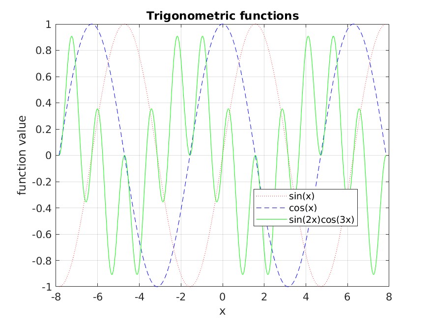
Consider the functions
\[ \sin(x) \] \[ \cos(x) \] \[ \sin(2x) \cos(3x) \]
on the domain
\[ -\frac{5}{2}\pi \le x \le \frac{5}{2}\pi \]
Below is a plot of these three functions on this domain produced using
the MATLAB plot command as well as other commands:
Generate a facsimile of this plot that reproduces all of its stylistic elements (line styles and colors, plot title, axes labels, legend) as closely as possible. Save a copy of the plot as a JPEG image.
You may find it convenient to implement your solution as a script If you do, ensure that your script file is created within the folder
Documents/MATLAB/
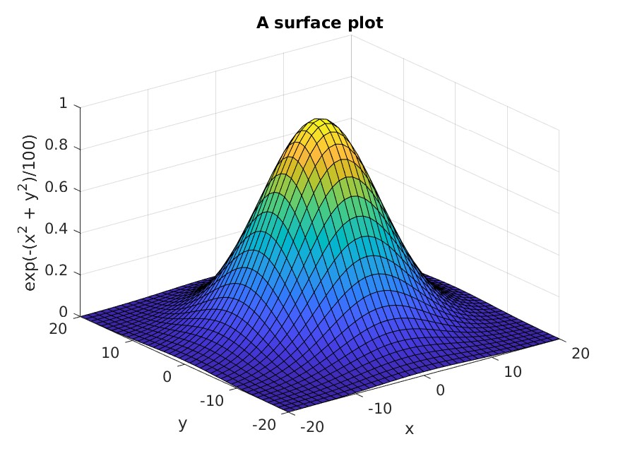
Try to reproduce the plot below, or create some other 3D plot of your own
design. Hint: Consider the MATLAB functions meshgrid and
surf.