Open a terminal window.
If you think "chaos" type
% touch /phys210/$LOGNAME/matlab/chaos
If you think "numerical artifact" type
% touch /phys210/$LOGNAME/matlab/numerical
CLASS DISCUSSION
In a terminal window, execute the following
% cd
% cp -r ~phys210/bounce .
% cd bounce
% ls

% make
Then open mbounce_fcn.c with your text editor and background it
% kate mbounce_fcn.c &

% gedit mbounce_fcn.c &
and start a Matlab session from that directory (~/bounce)
% mat
XForms/OpenGL based utilitiesWe will discuss three visualization utilities below:
xfpp3dxflat2d_rgbxvsAll of these
Because of the dependence on OpenGL, these applications will not run remotely on your PCs/laptops/Mac OSX etc., even if you have X11 support.
In other words, unless you want to install them on your own machines, which is possible if you're running OSX or Linux, you will have to use them in the lab.
If you are interested in installing them yourselves (but remember, this can not be done under Windows), send me an e-mail.
I have some basic utilities written in Matlab that may also be of use and I will try to add some more in the weeks to come.
Finally, it is important to bear in mind that all of these utilities read data that has been generated by an application, your term project scripts & functions for example, and each utility requires its data to be stored in a specific format. Part of the visualization package that I provide is a collection of Matlab functions that make it easy for you to output data to files in the form that the specific utility you will be using expects. In order to use the functions directly you will need to either:
Follow my suggestions (directives?) for how to represent the dependent variables in your project (including the CA projects, where the dependent variables are the states of all the lattice sites), as Matlab arrays. This includes the number of dimensions in the array, typically 3, and how the dimensions should be ordered.
Be prepared to copy the data in your representation to another array that does have the attributes expected by the function that you are using, and then supply the copy as an argument to the function.
Not surprisingly, the first option is definitely preferable in my opinion, and if you do decide to go the recommended route you will need to understand how your variables should be stored before you start to code. I've explained how this should be done for the N-body codes in pages 28-31 of the PDF notes, and if there's any confusion in your mind when your start to write your programs, ask me for help.
lookforUse
lookfor phys210-nbody
xfpp3dIMPORTANT
Again, note that all of the utilities described here must be executed from the shell, not in Matlab.
In a terminal window, change to your Matlab directory and then
copy the sample data file ~phys210/nbody/nbody3.dat to your
Matlab directory:
% cdm
% pwd
/phys210/phys210f/matlab

% cp ~phys210/nbody/nbody3.dat .
First, invoke xfpp3d with the -h option to get help for the utility
% xfpp3d -h

usage: xfpp3d [-h] [-c] [-s] [-w]

Displays animations of three dimensional particle motion.

  Options: -h   Displays this help message.
           -c   Enables user-specified coloring (RGB) of particles.
           -s   Renders particles as solid spheres.
           -w   Renders particles as wireframe spheres.

xfpp3d reads ASCII input from standard input in one of the following
two formats:

(Note that ! denotes the start of a comment.)


FORMAT 1: Default (all particles displayed in single, fixed color)

       <np>                            ! Number of particles
       <size_1>                        ! Display size of particle 1
       <size_2>                        ! Display size of particle 2
                   .
                   .
                   .
       <size_np>                       ! Display size of particle np
       <t_1>                           ! First display time
       <x_1_1>  <y_1_1>  <z_1_1>       ! Coordinates of particle 1 at t_1
       <x_1_2>  <y_1_2>  <z_1_2>       ! Coordinates of particle 2 at t_1

                             .
                             .
                             .
Note that all values can be real numbers (i.e. have a decimal
point) except for <np> which must be an integer.
Now we'll execute xfpp3d using the sample data file as input, and supplying
the option -c so that the particles are coloured:
WARNING
If you have output your nbody data with color information (i.e. so that
different particles, or groups have particles can have distinct
colors), which most of you eventually will, then you MUST use the
-c option!!
IMPORTANT
At the current time, xfpp3d only takes input from the standard input, so
use the input redirection operator < after the command name,
followed by the filename.
Also, background the command (& at the end), so that
you can continue to issue bash commands in the terminal session:
% xfpp3d -c < nbody3.dat &
INSTRUCTOR DEMONSTRATION OF xfpp3d USAGE ...
IMPORTANT
There is no facility to "rewind" or step back through
the time sequence of data. If you want to re-view the data, you
must exit the utility, and reexecute the xfpp3d command.
xfpp3d format: nbodyout & nbodyout1There are functions in ~phys210/matlab that can be used to output N-body data to a file in the format that xfpp3d requires.
Browse source
As usual, type
>> help nbodyout
>> help nbodyout1
for usage information.
As with all of the other course scripts and functions, and assuming that you are working on the lab computers, you should be able to use these directly in your programs
NOTE
The only difference between nbodyout and nbodyout1 is the following
nbodyout requires that the position array be dimensioned
r(np, 3, nt)
where np and nt are the number of particles and time steps,
respectively, and which is the form advocated in the lecture
notes.
nbodyout requires that the position array be dimensioned
r(3, np, nt)
WARNING
nbodyout and nbodyout1 will both overwrite the
output file specified in the argument list (if it exists),
so be sure to rename or move the existing file, should you want
to preserve its contents.
nbodyout: tnbodyoutBrowse source
This driver generates sample N-body data for a "mock" solar system and
outputs it using nbodyout for subsequent viewing with xfpp3d.
Note that you are welcome to copy and modify this script, or pieces of it, for your own purposes. Again, that applies to all of the course Matlab code base.
First, ensure that your Matlab session is executing in your Matlab directory
Run the script and verify that the data file tnbodyout.dat
was generated:
>> tnbodyout
>> ls tnbodyout.dat
tnbodyout.dat
Go to a terminal window, ensure that it's also executing in your
Matlab directory, then use xfpp3d to view the data:
% cdm
% xfpp3d -c < tnbodyout.dat &
Locate the functions and scripts for this topic using
>> lookfor phys210-ca
life.m and lifea.mThere is a huge amount of online information concerning this particular cellular automaton, invented many years ago by John H. Conway, including many applets that play the "game"; click HERE for an overview
life.m and lifea.mBrowse source
lifea is a so-called vectorized version: i.e. the code uses
whole-array operations rather than for loops (although any
implementation must use a loop for time-stepping). Vectorized
code generally leads to performance gains, sometimes very large
ones. This is especially true for octave which does yet have
Matlab's facility to recognize when loops that
are operating on arrays can be vectorized and then automatically
vectorize the code.
Ensure that the working directory for your Matlab session is your Matlab directory
>> cdm
and then execute the script
>> life

id_type = 0
nx =  50
ny =  50
nt =  200
life: Step 1 of 200
life: Step 2 of 200
life: Step 3 of 200
life: Step 4 of 200
life: Step 5 of 200
life: Step 6 of 200
life: Step 7 of 200
life: Step 8 of 200
life: Step 9 of 200
        .
        .
        .
latout: Wrote 140 of 200
latout: Wrote 150 of 200
latout: Wrote 160 of 200
latout: Wrote 170 of 200
latout: Wrote 180 of 200
latout: Wrote 190 of 200
latout: Wrote 200 of 200
latout: Wrote nx=50 ny=50 nt=200 to file=life.dat
ca.mThis is based on research done in the mid 1980's by Stephen Wolfram at about the time he began work on SMP the precursor to Mathematica (M) and Wolfram Alpha. To say that this man loves to program is no doubt what he would consider the understatement of all time: see his offical web site for more information.
Browse source and driver
Run driver
>> tca
xflat2d_rgbAs with xfpp3d, this program must be executed in the shell, not in
Matlab.
In a terminal window, change to your Matlab directory and verify that
there's a file life.dat that was created when you ran life in
Matlab.
% cdm
% ls life.dat

life.dat
If life.dat isn't there, go back to your Matlab session, use
the Matlab function cdm (which has the same name as the bash
alias that we have defined) to ensure that the Matlab working
directory is correct, and then run life
>> cdm
>> life
You should see life.dat in a listing of that directory
First get help for the application, using the -h option:
% xflat2d_rgb -h

   usage: xflat2d_rgb [-h]

   Displays animations of two dimensional binary lattices colored with
   arbitrary RGB values.

   xflat2d_rgb expects the following formatted input on standard input:

   <nx> <ny>                                     ! Dimensions of lattice
   <t>                                           ! FIRST display time
   <val(1,1)>   <R(1,1)>   <G(1,1)>   <B(1,1)>   ! Lat, RGB values for site (1,1)
   <val(2,1)>   <R(2,1)>   <G(2,1)>   <B(2,1)>   ! Lat, RGB values for site (2,1)
                        .
                        .
   <val(nx,1)>  <R(nx,1)>  <G(nx,1)>  <B(nx,1)>  ! Lat, RGB values for site (nx,1)
   <val(1,2)>   <R(1,2)>   <G(1,2)>   <B(1,2)>   ! Lat, RGB values for site (1,2)
                        .
                        .
   <val(nx,2)>  <R(nx,2)>  <G(nx,2)>  <B(nx,2)>  ! Lat, RGB values for site (nx,2)
                        o
                        o
                        o
   Lattice positions (1,1) and (nx,ny) correspond to the upper left and
   lower right positions of the display area respectively.

   Input is stream oriented so carriage returns are effectively ignored.
   Thus for example, the lattice values at a given time could appear on
   a single line, one per line, one row per line etc.
Now use xflat2d_rgb to visualize the output generated by life and
stored in life.dat.
IMPORTANT
As with xfpp3d, xflat2d_rgb only takes input from
the standard input: you must use the input redirection operator <
between the command name and the filename:
% xflat2d_rgb < life.dat &
INSTRUCTOR DEMONSTRATION OF xflat2d_rgb USAGE ...
As with xfpp3d, there is no facility to "rewind" or step back through
the time sequence of data. If you want to replay the evolution,
exit the utility, and reexecute the xfpp3d command.
First, if your CA has nstate states, use consecutive integers to represent
them, i.e.
0, 1, ..., nstate - 1
or
1, 2, ..., nstate
Since CA rules must always completely define how a cell in any possible state evolves to the next time step, based on its current state and the states of all the cells in its neighbourhood, which integers you use for which states are completely arbitrary. I.e. you must decide how you are going to enumerate the state, but if the integer values aren't contiguous, such as
0, 1, 3, 4
rather than
0, 1, 2, 3
then the output utility function latout, described below, will not
work properly.
Second, use a 3-dimensional array (called c here) to store your CA data.
Define/initialize the array as follows:
c = zeros(nx, ny, nt)
so that c has dimensions nx x ny x nt, where nx, ny, nt are
nx: the size of lattice in the x-directionnz: the size of lattice in the y-directionnt: the number of time steps in the simulationEnsure that the time dimension is the final one (the third) or you
will not be able to use latout directly.
For efficiency, you should definitely use zeros(...) as above
to create the 3d lattice before the simulation per se is started.
Third, define an array of RGB values that defines the colors which will
be used by xflat2d_rgb for all of the state values.
For example, if your model has four states, say, 1, 2, 3 and 4, and you want to use the colors red, green, yellow and white, respectively, for them, then define
rgb = [ [1.0 0.0 0.0]; [0.0 1.0 0.0]; [1.0 1.0 0.0]; [1.0 1.0 1.0] ];
i.e. rgb is an nstate x 3 array, where each row is an RGB (red-green-blue)
triple defining a color (each R, G or B value must be in the range
0.0 to 1.0).
Fourth, assuming that you have followed/implemented these "hints" (and
you should!), then once your script has completed the simulation, so
that each element of the array has been defined (i.e. all nx x ny x nt
elements have been assigned a state value), use
latout('ca.dat', c, rgb);
to write the CA data to a file (called ca.dat here, you can use
whatever name you wish), that you can then visualize via
% xflat2d_rgb < ca.dat
Remember to
xflat2d_rgb from the shell, not Matlab< followed by the filename to
feed that data in the file to the application.WARNING
latout will overwrite the output file (ca.dat in
this example) if it exists, so be sure to rename/move the
existing file, should you want to preserve its contents.
Fifth, in a Matlab session, use
>> help latout
for additional usage information for latout, and
>> type latout
to see the function definition
Locate the functions and scripts for this topic using
>> lookfor phys210-xvs
Store your FD solutions (so called grid functions) in arrays
that are dimensioned nx by nt, where nx is the number of
grid points in the spatial direction, and nt is the number of
time steps in the simulation.
For those of you solving the Schrodinger equation, note that you should implement your FDA using complex arithmetic. This will simplify the code and Matlab can equally well deal with complex quantities as it can with real ones. Then, for example, initialize the single dependent variable (field) for your problem using something like
nx = <whatever>
nt = <whatever>
psi = zeros(nx, nt)
You can then assign complex values to psi (typically one column at a
time), i.e. there is no need to explicitly tell Matlab that you will
storing complex numbers in an array. It is, however, always good
to preallocate an array like psi, which tends to be large, using
zeros.
xvs and plot can not visualize complex-valued directly, so you
will need to extract the real and imaginary components of psi and
plot them (as well as other quantities, such as the magnitude of
psi, the potential and the running integrand of the magnitude of
psi). This is easy to do with the builtin functions real and
imag, which like all of the basic Matlab functions, take any array
as the input argument, and return an array with the same dimension as
output.
xvsSince there are very few of you doing projects that involve the solution of time dependent PDEs in 1 space dimensions (so called 1+1 problems),
I will not demo xvs in the lab. Rather, I will direct those who are
doing the above projects to the available online documentation which
should be enough to get you going, and you can simply ask me for
help as you need it.
Also, although xvs can be a very powerful tool for this kind of work since
it was specifically designed for visualizing the output from FD
codes for 1+1 calculations, Matlab's built in plotting facilities,
combined with the rudimentary animation technique used in bounce
and your extension of it may well suffice for your work.
Note that xvs is also XForms/OpenGL based, so will only work in
the lab or on Linux/OSX with all of the appropriate software installed.
If you really want to try to install it on your own machine(s), I can
certainly try to assist as time permits.
xvs Documentation
xvs to perform convergence tests HERENOTE
You can use the twave script to generate some solutions to the wave
equation that you can then convergence test using the technique discussed
in the summer school as a warm up for your own testing.
xvsIMPORTANT
To use xvs you must add the following line to your bash startup
file ~/.bashrc
export XVSHOST=`hostname -f`
Note that the quotes surrounding hostname -f in the above
assignment of the environment
variable XVSHOST are backquotes
Remember that one needs to modify ~/.bashrc very carefully, since
syntactic errors in it can make it impossible for you to login,
or result in a crippled bash setup.
So until you develop expertise with this task follow these steps religiously:
Change to your home directory and make a backup copy of the startup file
% cd
% cp ~/.bashrc ~/.bashrc.O
confirming overwrite of ~/.bashrc.O should it already
exist.
Edit the file from the command line and in the background:
% gedit ~/.bashrc &
or
Editing the file in this way is important since the terminal
session from which you launch the editor will not be affected
by any changes you make to the startup file. Thus, if you encounter
some problem while editing ~/.bashrc that you can't resolve,
you can always restore the backup copy from that terminal and
things should be back the way that they were when you started:
% cd
% cp .bashrc.O .bashrc
where you will need to confirm overwrite.
Test the changes
Test the changes that you make by opening a new window and typing
% printenv XVSHOST
You should see the fully qualified host name of the machine that you are using, e.g.
cord.phas.ubc.ca
xvsStart xvs from the command line in a terminal window. xvs will
write diagnostic information to the terminal (standard output) from
time to time, but you generally won't need to be concerned with that.
xvsoutxvsout is a Matlab function that will write data from a 1+1
FD code that can then be sent to xvs using that Unix command
asctoxvs described in the next section.
Browse source and driver
Within a Matlab session, change to your Matlab directory and run the driver
>> txvsout

Running wave at level 7
wave: tmax=2
wave: level=7
wave: lambda=0.5
wave: al=1
wave: x0l=0.45
wave: deltal=0.05
wave: ar=0.5
wave: x0r=0.55
wave: deltar=0.1

wave: nx=129
wave: delx=0.0078125
wave: nt=513
wave: delt1=0.00390625
wave: delt=0.00390625
wave: u [129 513]
wave: x [129]
wave: t [513]
wave: Number of time steps to take: 513

wave: Step   50  100  150  200  250  300  350  400  450  500  Done.

Elapsed time is 0.054103 seconds.

Calling xvsout to write to txvsout.dat
Checking for txvsout.dat
-rw-r--r-- 1 phys210f phys210f 3.2M Nov  9 21:06 txvsout.dat

Done.
xvs: asctoxvsInvoke asctoxvs from the bash command line, not in a Matlab session.
Used without arguments it will display a usage message:
% asctoxvs

Synopsis:
  Sends an ASCII file to the xvs visualization server

Usage:
  asctoxvs file [xvsname]

  file    -- file to be transmitted
  xvsname -- xvs name for data [defaults to file]

File Format:
        .
        .
        .
To send the data in a file previously created using xvsout simply
type asctoxvs followed by the filename. For example, assuming
that
~/.bashrc so that XVSHOST is
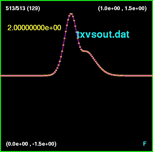
set to the hostname as described above.xvs from the bash command line txvsout script in Matlab as described abovethen if you type the command sequence
% cdm
% asctoxvs txvsout.dat
a window looking like the following should appear in the xvs app, and you
can view and manipulate the data as described in the online documentation
available via the links given above.